Abstract
Diffeomorphic registration using optimal control on the diffeomorphism group and on shape spaces has become widely used since the development of the large deformation diffeomorphic metric mapping (LDDMM) algorithm. More recently, a series of algorithms involving sub-Riemannian constraints have been introduced in which the velocity fields that control the shapes in the LDDMM framework are constrained in accordance with a specific deformation model. Here, we extend this setting by considering, for the first time, inequality constraints in order to estimate surface deformations that only allow for atrophy, introducing for this purpose an algorithm that uses the augmented Lagrangian method. We prove the existence of solutions of the associated optimal control problem and the consistency of our approximation scheme. These developments are illustrated by numerical experiments on simulated and real data.
Keywords: diffeomorphic registration, medical imaging, optimal control, constrained optimization
AMS subject classifications. 58D05, 49N90, 49Q10, 68E10
1. Introduction.
Over the last couple of decades, multiple studies have provided evidence of anatomical differences between control groups and cognitively impaired groups at the population level for a collection of diseases, including schizophrenia, depression, Huntington’s, and dementia [45, 19, 11, 46, 66, 53, 1, 36, 52, 64, 41]. In the particular case of neurodegenerative diseases, a repeated objective has been to design anatomical biomarkers, measurable from imaging data, that would allow for individualized detection and prediction. This goal has become even more relevant with the recent emergence of longitudinal studies involving patients at early stages, or “converters,” who showed that, when the effect is measured at the population level, anatomical changes caused by diseases like Alzheimer’s or Huntington’s were happening several years before cognitive impairment could be detected on individual subjects.
Shape analyses from medical imaging data rely most of the time on a registration step that places the subjects’ anatomies in a common coordinate system, often associated with a template, or average shape, to which all images are coregistered [15, 56, 58, 8, 5, 6, 9, 10, 38, 39, 59, 60]. A large number of registration methods have been proposed in the literature, with an extensive survey proposed in [51], including more than 400 references for image registration alone. Surface registration has also been extensively developed [27, 26, 57, 18, 34, 37, 4, 61, 68, 7, 13, 35, 67, 12].
We focus in this paper on surface registration using the large deformation diffeomorphic metric mapping (LDDMM) algorithm, which has been used extensively to analyze shape variation in regions of interest (ROIs) represented by triangulated surfaces. While some of its main advantages are its flexibility and its ability to render smooth, diffeomorphic, free-form shape changes, there are situations in which prior information is available and should be used to enhance the results of the shape analysis and make it more robust to noise. In this paper, we focus on situations in which no tissue growth is expected to occur. In such contexts, it is natural to ensure that shape analysis should only detect atrophy, even when noise and inaccuracy in the ROI segmentation process may lead in the other direction. (Here, we mean “atrophy” in the general sense of local volume loss.) In this paper, we introduce an atrophy-constrained registration algorithm, which includes some of the ideas introduced in [2], while extending them to inequality constraints associated to the problem we consider. The primary application of the proposed method is for longitudinal data (time series), for which our approach can be seen as a generalization of monotonic nonlinear regression. This adds a new tool to the growing set of methods developed for regression in infinite-dimensional shape spaces, which include, among others, kernel regression, geodesic regression, polynomial regression, and shape spline regression [16, 43, 55, 20, 21, 30, 31, 29, 32, 40].
The atrophy-constrained registration algorithm will be described in section 2, with our numerical approach discussed in section 3. Some theoretical results on existence of solutions and consistency of discrete approximations are provided in section 4. An extension of the algorithm to include affine alignment is provided in section 5. The application of this algorithm to time series is discussed in section 6. Finally, experimental results are provided in section 7.
2. Atrophy-constrained LDDMM.
Although time series, discussed in section 6, will be the primary application of the atrophy-constrained framework, we will start by discussing the approach with the standard two-shape case (“template to target”), since it includes all the new developments in a simpler context.
2.1. Continuous optimal control problem.
The LDDMM algorithm implements an optimal control strategy in which a template surface S0 is “driven” toward a target surface S1 via a time-dependent process t ↦ S(t), with S(0) = S0. This is achieved by minimizing
| (1) |
subject to the state equation dS/dt = v(t, S(t)), where v is a smooth velocity field on . By , we mean a functional norm in a reproducing kernel Hilbert space (RKHS) V, which we will assume to be embedded in (the completion, for the standard supremum norm of up to p derivatives, of the space of compactly supported infinitely differentiable vector fields) with p ≥ 1. This space can, for example, be defined as the Hilbert completion of
(originally defined for smooth vector fields), where A is a differential operator. A typical example is A = (Id − Δ)k, where Id is the identity, Δ is the Laplacian operator, and k is large enough to ensure that required Sobolev inclusions hold. In the general case, let be the Hilbert duality mapping, so that is the linear form w ↦ ⟨v , w⟩V, and let . The reproducing kernel of V, also denoted , is a mapping defined on , with values in (the set of 3 × 3 real matrices) such that, letting denote the ith column of , the vector field belongs to V for all with, for all v ∈ V, , the ith coordinate of v(y). To simplify the notation, we will assume in this paper that is a scalar kernel, i.e., that it takes the form , where K is scalar valued.
The function D in (1) is a measure of discrepancy that penalizes the difference between the controlled surface S(·) at the end of its evolution and the target surface S1. Among the measures introduced in the literature in combination with the LDDMM algorithm, the most convenient computationally are designed as Hilbert-space norms between surfaces considered as linear forms over spaces of smooth structures. The “simplest” example, linear forms on smooth scalar functions arising from integrating functions over surfaces, yields the “measure matching” cost introduced in [24, 25]. “Current matching,” introduced in [23, 57], results from integrating smooth differential forms over oriented surfaces. More recently, varifold-based cost functions [12] were designed, in which functions defined on (the Grassmannian manifold of two-dimensional (2D) spaces in ) are integrated over the surface. Details on these cost functions, their discrete versions on triangulated surfaces, and the computation of their gradient are provided in the cited references. To focus the discussion, we will here assume that D is based on the current-matching norm, which is defined as follows. Given a positive definite kernel χ, define the “dot product” between two oriented surfaces by
| (2) |
where , refer to the area forms on S and S′, and NS, NS′ to the oriented normals. We will then use the cost function (between two oriented closed surfaces S and S′)
| (3) |
where λ ≥ 0. The first part of the cost function is the current norm introduced in [57]. The second part (weighted by λ) compares the interior volumes of the surfaces. This term is redundant (since a vanishing current norm implies that the surfaces are identical), but has a stabilizing effect in the atrophy-constrained estimation.
Interpreting (1) in optimal control language, v is the “control,” S is the “state,” and v is optimized in order to bring the state near a desired endpoint. With this construction, each point x0 in S0 is registered to a point x(t) = φ(t, x0) in S(t) that evolves according to the differential equation dx/dt = v(t, x), with x(0) = x0. The overall evolution is diffeomorphic, e., for each time t, φ(t, ·) can be extended to a smooth invertible transformation with smooth inverse on .
To define our atrophy constraints, we assume that surfaces are closed and oriented. We let N0(x0) be the outward-pointing unit normal to S0. An outward-pointing normal to S(t) at x = φ(t, x0) is then given by
| (4) |
where dφ(t, x0) denote the differential of y ↦ φ(t, y) at y = x0 (a 3 × 3 matrix), with the “−T” exponent indicating the transposed inverse. Note that N(t, x) does not necessarily have norm one.
We can express the atrophy constraint by the fact that the surface evolves inward at all points, i.e., by v(t, x)TN(t, x) ≤ 0 for all x ∈ S(t) and t ∈ [0, 1]. Adding this constraint to the original surface-matching LDDMM problem leads to the atrophy-constrained problem of minimizing
subject to ∂tS = v(t, S(t)), v(t, x)TN(t, x) ≤ 0, x ∈ S(t).
We now reformulate this problem under the assumption that S0 is parametrized with an embedding , where M is a 2D Riemannian manifold. This is no loss of generality, since one can always take M = S0 and q0 = identity. It will also be useful, when discussing discrete approximations, to relax the atrophy constraint to the form v(t, x)TN(t, x) ≤ ε∣N(t, x)∣, x ∈ S(t), which allows for a small amount of expansion, with normal velocity less than ε. Given this, we take parametrizations as state variables, together with functions , and solve the following.
Problem 1. Minimize
| (5) |
| (6) |
Here, with a slight change of notation, N0(m) is the outward-pointing unit normal to S0 at q0(m). N(t, m) is then an outward-pointing (not necessarily unit) normal to S(t) = q(t, M) = φ(t, S0) at q(t, m). The third equation in the constraints is the time derivative of (4).
2.2. Discrete approximations.
We now assume that surfaces are triangulated, so that parametrizations are replaced by pairs (q, F), where is a set of n vertices (where n depends on S) and F ⊂ {1, … , n}3 provides the list of indices of vertices that form the triangular faces.
We assume that these surfaces are oriented, so that an edge that belongs to two faces is oriented in different directions in each face. If q = (q1, … , qn) and f = (i, j, k) ∈ F, we let S(q, f) denote the closed triangle with vertices (qi, qj, qk). We also let c(q, f) = (qi + qj + qk)/3 be the center of mass and
| (7) |
be the area-weighted normal, this expression being invariant by circular permutation of i, j, and k (N(q, f) is oriented according to the normal to the face, with norm equal to the area of the face). From this we define the area-weighted normal at a vertex qk by
| (8) |
and let N(q, F) = (N1(q, F), … , Nn(q, F)). Finally, we let S(q, F) be the associated piecewise-triangular surface, namely,
To define a discrete version of Problem 1, we introduce state variables q = (q1, … , qn) and N = (N1, … , Nn), initialized with an initial triangulation (q0, F0). We also assume a target surface (q1, F1). The discrete problem will minimize
Here, Dδ is a discrete approximation of D in (3) in which the dot product between triangulated surfaces is replaced by
| (9) |
(so that χ is approximated by a constant value on each face). Volumes of triangulated surfaces are computed exactly. (We here refer to the above problem as “discrete” even though the continuous time variable remains in its formulation, to reflect the fact that we passed from an optimal control problem with an infinite-dimensional shape space to a standard finite-dimensional one.)
Given that the endpoint cost and the constraints depend on v only through the configurations q(t), one shows, using standard RKHS reductions, that the optimal v takes the form
where K is the reproducing kernel of V. Using this, the previous problem reduces to the following.
Problem 2. Minimize
| (10) |
| (11) |
However, in the discrete case, it is possible to avoid the introduction of N as a state variable and solve the following instead.
Problem 3. Minimize
| (12) |
| (13) |
Note that the apparent simplification is balanced by the fact that the constraint becomes a more complex function of the state and controls, with Nk (q, F0) given by (7) and (8).
3. Numerical method.
Problem 3 is solved using augmented Lagrangian methods, introducing, as described in [44], slack variables to complete inequality constraints. More precisely, let
and let C(q) = (Ckl(q), k, l = 1, … , n) be the associated n × 3n matrix. Let K(q) be the 3n × 3n matrix formed from blocks (). For a vector u, let u+ denote the vector formed with the positive parts of each of the coordinates of u. Let ∣N∣ denote the n-dimensional vector with kth coordinates equal to ∣Nk∣.
The augmented Lagrangian is defined by
| (14) |
Here, the parameter μ is a small positive number, is a Lagrange multiplier, and q is considered as a function of α via the state equation ∂tq = K(q)α. The augmented Lagrangian optimization procedure iterates the following steps (starting with initial values (α0, λ0)):
Minimize α ↦ F(α, λn) to obtain a new value αn+1 (and qn+1 via the state evolution equation).
Update λ with λn+1 = (μλn − C(qn+1)αn+1 + ε∣N∣)+ /μ.
If needed (e.g., if ∣(C(qn+1)αn+1 − ε∣N∣)+∣ is larger than a threshold δn), replace μ by a smaller number, ρμ, with ρ < 1.
The most expensive step is, of course, the first one, which requires solving an optimal control problem equivalent in complexity to the unconstrained problem. The computation of ∇αF(α, λ) (the gradient of F with respect to α) uses a back-propagation algorithm, also called the adjoint method. Since similar computations are described in multiple places [57, 65, 14, 4], we briefly summarize it here.
Given α, compute the associated state q via ∂tq = K(q)α and evaluate the matrix C(q).
-
Introduce a costate , t ∈ [0, 1], defined by
(Note that the square of the positive part of a number is differentiable.)
Define .
Remark. Ensuring that the total volume of the surface decreases (instead of enforcing inward motion at every point) can be done very similarly to the full atrophy constraint, using the single constraint or, after reduction,
where Nk is given by (8). It is important here to use the area-weighted normal to discretize the continuous constraint , which provides the derivative of the total volume with respect to time. This constraint can be rewritten as , where 1n is the n-dimensional vector with all coordinates equal to 1. The reformulation of the augmented Lagrangian method for this scalar constraint is straightforward and left to the reader.
4. Existence of solutions and convergence.
The following theorems address two important properties of the proposed method. The first one shows that solutions of the constrained problem within our space of interest exist, and the second one considers the issue of consistency of the discretization approach, showing that under suitable assumptions, the solutions obtained with discrete surfaces converge to solutions of the continuous problem. These results are proved in the appendices.
Theorem 1. Assume that V is continuously embedded in for p ≥ 2 and that the data attachment term D is such that φ ↦ D(φ(S0), S1), defined over all Cp-diffeomorphisms φ such that φ − , is continuous for the uniform Cp convergence over compact sets. Then Problems 1, 2, and 3 always have an optimal solution v ∈ L2(0, 1; V).
The assumption on D applies to the one defined in (3) as soon as p ≥ 1.
We now introduce some assumptions to address the consistency of discrete approximations. We say that a sequence of triangulations ((qn, Fn)) converges nicely to a surface S of class C2 if there exists an n ≥ n0 such that the following conditions are satisfied.
The vertices of Sn belong to with for k = 1, … , mn.
-
The triangulations are nested:
In particular, we can order the collection of all vertices of the triangulations in a countable sequence (q1, q2, …), and for each qj there exists an integer nj such that qj is a vertex in qn for all n ≥ nj.
The maximum edge length in (qn, Fn) goes to 0.
-
If η(qn, f) is the length of the largest edge of a face f, the ratio
f ∈ Fn, is bounded away from 0 (uniformly in n).
The triangulations are close enough to S to ensure that every point x ∈ S(qn, Fn) has a unique closest point ξ(x) on S, such that ξ is onto.
These hypotheses imply the convergence of normals as follows [42].
-
In addition
when n goes to infinity, where N is the unit normal to S.
We have the following result.
Proposition 1. Assume that (qn, Fn) converges nicely to S and (, ) converges nicely to S1. Then
when n goes to infinity, where D and Dδ are defined in (3), (2), and (9).
We can now state our consistency theorem.
Theorem 2. Fix ε∞ > 0, and assume that V is continuously embedded in for p ≥ 2. Let S0 and S1 be two C2 surfaces, and let (), () be two sequences of triangulations that converge nicely to S0 and S1, respectively. Then there exists a decreasing sequence of real numbers εn > 0 with εn → ε∞, such that if vn ∈ L2(0, 1; V) solves Problem 2 with ε = εn, initial surface , and target , then the sequence is bounded in L2(0, 1; V), and any weak limit point v* of vn is a solution to Problem 1 with ε = ε∞.
5. Affine alignment.
Because the RKHS V is embedded in , vector fields v ∈ V vanish at infinity. This implies, in particular, that affine transformations do not belong to this Hilbert space, and that the diffeomorphic registration does not incorporate any rigid alignment. If such an alignment is needed, one can include it in the optimal control framework by completing the control with the corresponding vector fields.
Let the registration be computed over , where G is a subgroup of , ⋉ referring to the semidirect product extending G with translations to obtain affine transformations. Let g be the Lie algebra of G, with basis E1, … , Eh. Instead of v ∈ V, we use a control given by (v, β1, … , βh, τ) with and , and the state equation
| (15) |
with associated cost for some nonnegative numbers c0, c1, … , ch. The extension of the numerical procedure to this setting is rather straightforward and not detailed here. It is also natural to include non-Euclidean affine components in the atrophy constraint v · N ≤ ε∣N∣.
The Euclidean case (rigid correction) is, however, the most interesting for application. This corresponds to G = SO3, the rotation group (so that h = 3). We will assume that Euclidean transformations act as isometries on V, which means that, for all v ∈ V, R ∈ SO3, , the vector field also belongs to V and . Euclidean-invariant RKHSs of vector fields are extensively described in [22], to which we refer the reader for more details. In the case of scalar kernels , Euclidean invariance implies that K is a radial kernel, i.e., that K(x, y) = γ(∣x − y∣2) for some function γ (additional conditions on γ are needed to ensure that K is a positive kernel; see [22]). Assume finally that the endpoint cost D is invariant by the Euclidean transformation: D(S, S′) = D(RS + b, RS′ + b). In this case, the optimal control problem (using c0 = ⋯ = c3 = 0) that minimizes in v, β, τ, subject to
| (16) |
is equivalent to minimizing in , R1, b1, subject to
| (17) |
via the change of variable , , , with , , R1 = R(1)−1, and b1 = −R(1)−1b(1). In other words, Euclidean registration via optimal control using (16) is equivalent to the original atrophy-constrained LDDMM optimizing its target over an orbit under the action of rigid transformations.
Note that c0 = ⋯ = ch = 0 should not be used with general affine transformations when noncompact components of the affine group are added to rotations. Intuitively, this would allow small deformations to be scaled up to larger ones at zero cost, and one can conjecture that the associated optimal control problem has no solutions and admits minimizing sequences of controls with vanishing cost at the limit. The equivalence with a problem in which the target is allowed to vary over its orbit via affine transformations is not true either for groups larger than the Euclidean one, essentially because invariant kernels do not exist in such cases.
Some attention should be paid to the discretization in time t, in particular in the rigid case. In our implementation, we use a simple Euler scheme to discretize the equation ∂tq = v(t, q); i.e., we take q(t + δt) = q(t) + δt v(t, q(t)). When using rigid registration, however, we take, with a skew-symmetric matrix,
to discretize ∂tq = v(t, q) + Aq + τ, with the explicit expression , for a 3 × 3 skew-symmetric matrix U. This ensures that the rigid registration remains a displacement, even for large values of the coefficients βl, which are made possible by the absence of cost on this transformation.
6. Application to time series.
Longitudinal studies generally include more than one followup scan, and we now extend our algorithm to the case of multiple targets observed at successive times. We still have a baseline surface S0 and now assume p followup surfaces S1, … , Sp. A direct generalization of the previous approach replaces (5) in Problem 1 by
| (18) |
where 0 < t1 ≤ ⋯ ≤ tn = 1 are attachment times, which can be fixed a priori (e.g., tk = k/n) or also optimized. The expression in (18) should be minimized, starting from a baseline S0, with the same constraints as in the single-target case.
As pointed out in [48, 49, 33, 3], this formulation of longitudinal registration (with or without atrophy) gives a special role to the baseline image and creates a bias in the way the information is obtained by breaking the symmetry within the acquisition and segmentation protocols that provided the images or surfaces. To address this, we add an extra error term, D(S(t0), S0) with t0 = 0, making the sum start at k = 0 in (18). The trajectory baseline, S(0), becomes a new variable to estimate. To ensure that the topology of the estimated trajectory remains consistent with the data (as was originally enforced by S(0) = S0), we assume that S(0) is a diffeomorphic transformation of another surface (a template) of known topology. Letting denote the template, this leads to the minimization of
| (19) |
where λ is a regularization parameter and controls a smooth deformation between the template and the initial point of the trajectory, S(0). More precisely, we let , where is a template-to-baseline trajectory satisfying and . The cost function is then minimized in the pair of chained controls (, v). While atrophy constraints remain applicable to v, no such constraint is enforced on . This algorithm has been implemented in Python, and examples of trajectories are provided in the next section.
7. Experimental results.
We now present experiments that compare time series, as described in section 6. We start with simulated sequences, which we use to analyze the performance of the method in handling noise, as well as possible bias that could occur from the asymmetric constraint (atrophy vs. expansion). We will then describe real data results using the BIOCARD dataset.
7.1. Simulated sequences.
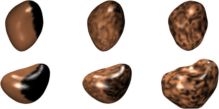
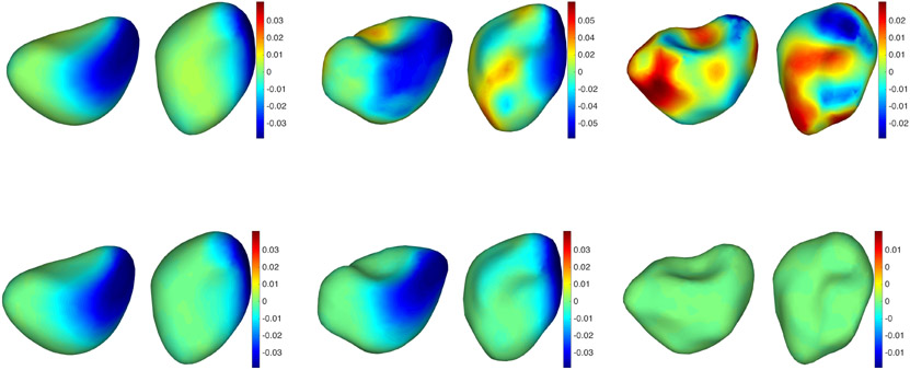
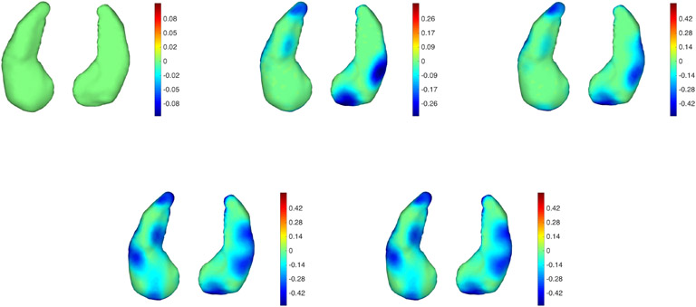
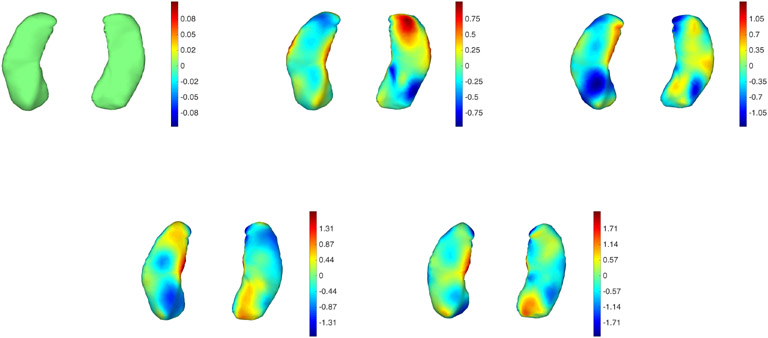
We ran a controlled experiment, using as a baseline a manually designed shape depicted in Figure 1. The surfaces used in this experiment are generated as follows. We built a template surface by hand using digital sculpting software. For each time t in the sequence, an expansion/atrophy field is defined on a template surface, taking the form z(t) = ta + ε(t), where a ≤ 0 is an atrophy pattern visualized in the first column of Figure 1, and ε(t) is a smoothed white noise on the surface (see the second and third columns of Figure 1). The template surface is then evolved along its normal, at a speed proportional to z(t) weighted by the mean curvature, yielding the surface at time t. We generate one baseline surface at t = 0 (which is only subject to noise) and nine followup surfaces for t = 1, 2, … , 9. Only the odd-numbered followup surfaces were used in registration. We ran three experiments: atrophy with low noise, atrophy with high noise, and noise only.
Figure 1.
Baseline surfaces used in the simulation study. Atrophy will be applied on the darkest area and expansion on the lightest one (the baselines are obtained after only adding noise). From left to right: Original atrophy pattern (before adding noise), atrophy pattern with small noise, atrophy pattern with large noise. The second row provides alternate views of the same surfaces. The dark area was formed by taking the intersection of the surface with a half plane, slightly smoothed by the heat equation. The noisy patterns were generated by adding white noise to the original function, before applying the heat equation again.
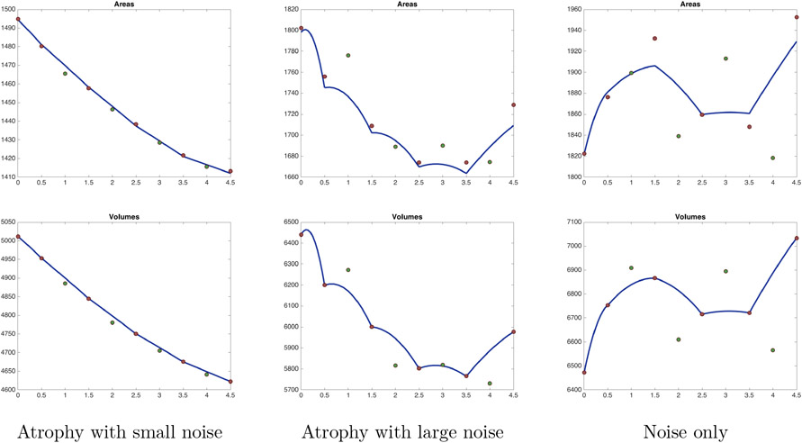
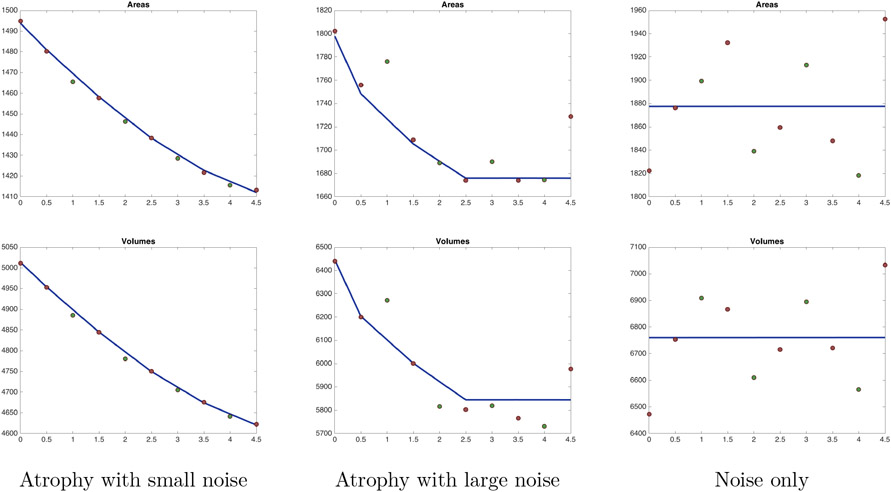
Figures 2 and 3 track surface areas and volumes along the estimated trajectories. Note that volumes almost coincide with the one obtained on the trajectories, as a consequence of the penalty term introduced in (3). Because no template surface was available for this experiment, we simply repeated the baseline, making it take the roles of both template and first target S0. In the small noise with atrophy setting, the introduction of constraints has little effect on the results. The difference between the two approaches is, however, notable for large noise in which the unconstrained trajectories closely follow the data, especially the final “outlier,” while the atrophy-constrained trajectories remain constant at the end to avoid expansion. This is confirmed in the pure noise experiment, for which the atrophy-constrained solution is constant at an average level, while the unconstrained one follows the noisy data.
Figure 2.
Areas and volumes along trajectories estimated without the atrophy constraint. For the three considered cases, the surface area is plotted in the first row, and the volume in the second row. The blue curve provides values computed for the optimized trajectory over time. Red dots are values for targets that have been included in the cost function. Green dots are for targets that were left aside.
Figure 3.
Areas and volumes along trajectories estimated with the atrophy constraint. Refer to Figure 2 for additional details.
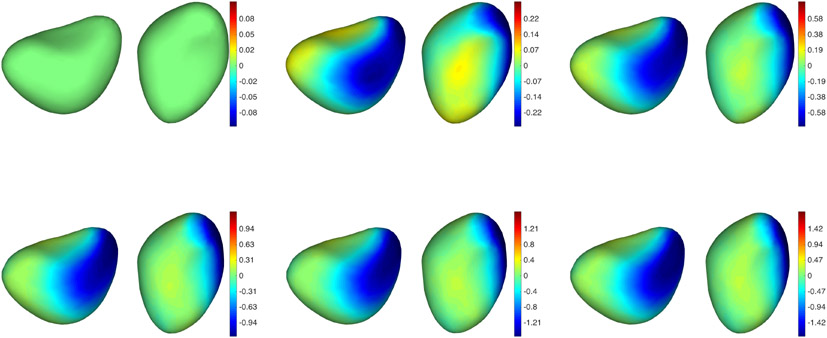
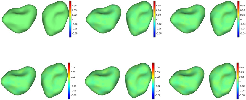
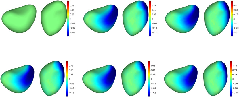
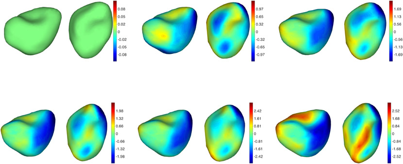
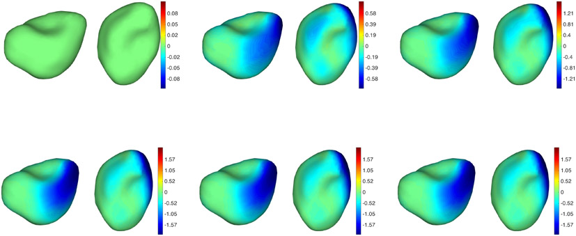
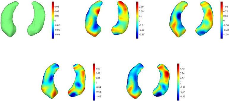
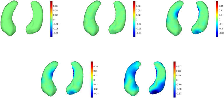
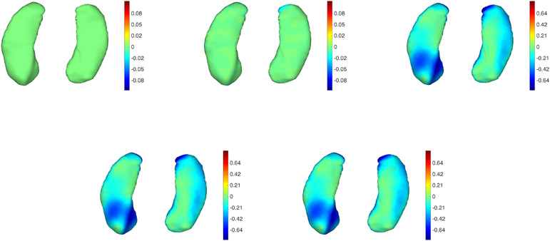
In Figures 4 to 9, we provide a more detailed illustration of the regions on the considered shapes over which atrophy was detected. These graphs provide the signed normal displacement of each point on the surfaces at different steps along the estimated trajectories, when performing longitudinal registration with and without atrophy constraint (all signals are scaled to their respective color maps, who are provided in the figures). In the small noise situation (Figures 4 and 5), the two approaches exhibit only mild differences. These differences become more visible when the original atrophy pattern is perturbed by a more significant amount of noise (Figures 6 and 7). In this situation, the unconstrained trajectories reflect the noisy atrophy/expansion pattern, while the constrained ones estimate atrophy on a region which is very close to the originally designed one. Some atrophy is also detected in other regions, too, but to a much lesser extent. The unconstrained trajectory also provides a highly variable pattern in the pure noise experiments (Figures 6 and 7), while the constrained one estimates a constant trajectory, estimating an “average” surface with very small variations over time. The same effects are summarized in Figure 10, in which pointwise atrophy rates (slope of the regression line of displacement against time for every point in the surfaces) are depicted for the various considered cases. Here again, both unconstrained and constrained methods provide similar results when the noise is small, and differ significantly for large noise, especially in the pure noise situation.
Figure 4.
Simulated data: Surfaces with small random deformation and atrophy tracked without atrophy constraints. From left to right and top to bottom: Baseline followed by 5 points in the trajectory. Two views are provided for each time point. The color map is proportional to the displacement (red: outward; blue: inward).
Figure 9.
Simulated data: Surfaces with large random deformation tracked with atrophy constraints. The target sequence is the same as in Figure 8. See Figure 4 for additional details.
Figure 5.
Simulated data: Surfaces with small random deformation and atrophy tracked with atrophy constraints. The target sequence is the same as in Figure 4. See Figure 4 for additional details.
Figure 6.
Simulated data: Surfaces with large random deformation and atrophy tracked without atrophy constraints. See Figure 4 for additional details.
Figure 7.
Simulated data: Surfaces with large random deformation and atrophy tracked with atrophy constraints. The target sequence is the same as in Figure 6. See Figure 4 for additional details.
Figure 10.
Atrophy rates for simulated data. From left to right: atrophy with small noise, atrophy with large noise, and noise only. First row: trajectories estimated without constraint. Second row: trajectories estimated with constraint.
7.2. BIOCARD data.
We here provide a similar set of illustrations for time series extracted from the BIOCARD dataset. The BIOCARD study [41, 50, 47] is a longitudinal study of Alzheimer’s disease (AD) in which subjects have been continuously followed for more than 20 years. BIOCARD has, compared to other longitudinal studies on AD, the distinction of having only included individuals who had no sign of cognitive impairment at baseline. The BIOCARD study was initiated in 1995 with the subjects having received their most recent cognitive assessment in 2012, resulting in about one-fourth of the group being diagnosed with mild cognitive impairment (MCI) or AD.
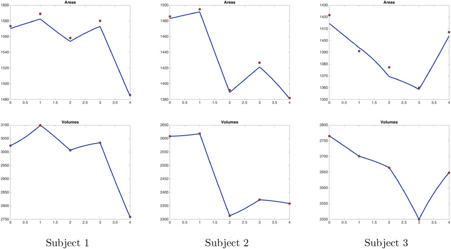
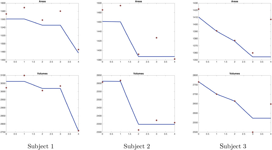
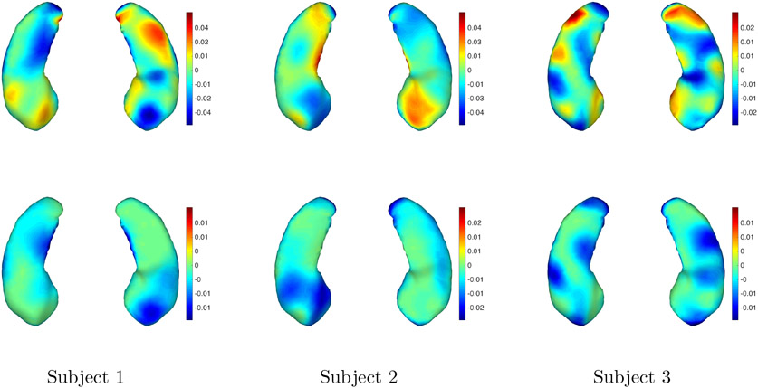
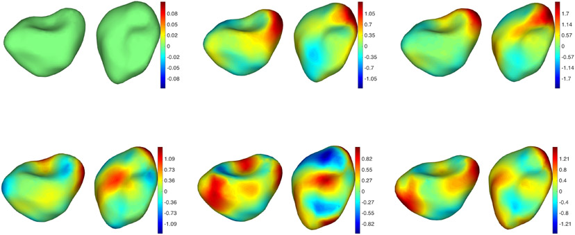
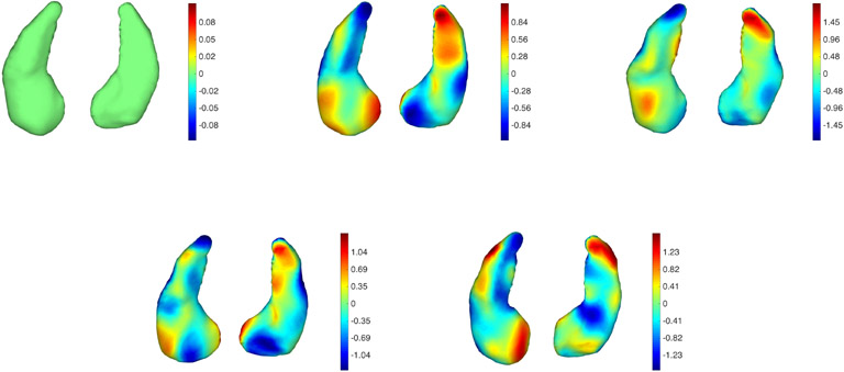
We selected three subjects (labeled subject 1 to 3) from this dataset, with five scans available for each of them (one baseline and four followup). Like most subjects in the cohort, these subjects were cognitively healthy at scan time. As in the previous section, we first display summary plots that trace the evolution of area and volume along the trajectories (Figures 11 and 12). We then show pointwise atrophy/expansion mapped on surfaces with and without constraints (Figures 13 to 18), followed by a visualization of the atrophy rate (Figure 19).
Figure 11.
Areas (top) and volumes (bottom) of surfaces tracked without atrophy constraint. Each column represents a subject from the dataset. Red dots provides values of area or volume for the original sequence.
Figure 12.
Areas (top) and volumes (bottom) of surfaces tracked with atrophy constraint. Each column represents a subject from the dataset. Red dots provides values of area or volume for the original sequence.
Figure 13.
Subject 1 from the BIOCARD dataset tracked without atrophy constraints. From left to right and top to bottom: Baseline followed by 4 points in the trajectory. Two views are provided for each time point. The color map is proportional to the displacement (red: outward; blue: inward).
Figure 18.
Subject 3 from the BIOCARD dataset tracked with atrophy constraints. The sequence is the same as in Figure 17. See Figure 13 for additional details.
Figure 19.
Rate of atrophy/expansion estimated for subjects 1 to 3. Two views of the same surface are provided in each frame. The first row provides values computed from the trajectories estimated without atrophy constraint, and the second from those estimated with the constraint.
Obviously, there is no ground-truth information that we can rely on to validate these results. The use of an atrophy-constrained model in this setting must be justified by prior expectations on the impact of the disease. While some volume gain in the brain can sometimes be observed, due to medication or inflammation, it is widely believed that AD affects brain regions like the hippocampus with synaptic or neuronal loss, which results in atrophy. Whether possible observed expansion is due to imaging or segmentation noise, or to other factors, it makes sense to try to disregard them and focus on atrophy. For the examples provided in this paper, the shape evolution appears much simpler and regular when estimated using atrophy constraints than without. The pattern of shape change that is observed in the results obtained with the former approach forms a subset of those provided by the latter, and seem to focus on changes that consistently occur over the 10-year period during which the scans were acquired.
8. Discussion.
In this paper, we have introduced a new approach targeting atrophy in the registration of longitudinal data, in view of applications to the analysis of neurodegenerative diseases. We have formulated the problem via constrained optimal control and proposed an algorithm that combined the adjoint method in optimal control with augmented Lagrangian methods. We also provided theoretical results on the existence of solutions for the problems, and on the consistency of our numerical scheme for approaching the solution.
Figure 8.
Simulated data: Surfaces with large random deformation tracked without atrophy constraints. See Figure 4 for additional details.
Figure 14.
Subject 1 from the BIOCARD dataset tracked with atrophy constraints. The sequence is the same as in Figure 13. See Figure 13 for additional details.
Figure 15.
Subject 2 from the BIOCARD dataset tracked without atrophy constraints. See Figure 13 for additional details.
Figure 16.
Subject 2 from the BIOCARD dataset tracked with atrophy constraints. The sequence is the same as in Figure 15. See Figure 13 for additional details.
Figure 17.
Subject 3 from the BIOCARD dataset tracked without atrophy constraints. See Figure 13 for additional details.
Acknowledgments
The research of the authors was supported in part by grants from the National Institutes of Health (U01-AG03365, P50-AG005146, R01-EB017638, R01-NS084957, P41-EB015909), the Office of Naval Research (ONR-90048203), and the National Science Foundation (ACI-1053575) for the Computational Anatomy Gateway via Extreme Science and Engineering Disc overy Environment (XSEDE). This work was partially supported by DCM 1335035.
Appendix
Appendix A.
Proof of Theorem 1. This theorem is proved along the same lines as similar statements addressing the existence of solutions for LDDMM problems [54, 17, 62, 63, 2]. We only provide a proof for Problem 1, since Problems 2 and 3 are addressed in a very similar way.
Let vn be a minimizing sequence. The boundedness of vn in L2(0, 1; V) implies that (extracting a subsequence if needed) vn converges weakly in this Hilbert space to a limit v (with a norm in L2(0, 1; V) no larger than the lim inf of the norms of vn). This, in turn, implies that the associated flows of diffeomorphisms φn (associated to vn) and their first p spatial derivatives converge uniformly (in time and space) over compact sets to φ (associated to v) and its first p derivatives [17, 62]. One gets from this that D(φn(1, S0), S1) converges to D(φ(1, S0), S1).
Letting (qn, Nn) denote the state in Problem 1 associated with the control vn, we have qn(t) = φn(t, q0), Nn(t) = dφn(t, q0)−TN0, therefore converging to q(t) = φ(t, q0) and N(t) = dφ(t, q0)−T N0 when n → ∞. This and the upper bound of the L2(0, 1; V)-norm of v imply that the cost function is minimized at v.
We now show that v(t, q(t, x))T N(t, x) ≤ ε∣N(t, x)∣ for all x ∈ M and almost all t ∈ [0, 1]. Fixing x and writing
one easily deduces from the facts that vn converges weakly to v, dvn is uniformly bounded, and qn and Nn converge uniformly to q and N that vn(t, qn(t, x))TNn(t, x) converges weakly to v(t, q(t, x))TN(t, x) in . This implies that v(t, q(t, x))TN(t, x) ≤ ε∣N(t, x)∣ for almost all t (the set of nonpositive a.e. functions is a closed convex set in L2 and therefore also weakly closed). By considering a countable dense set of x’s, and using the fact that x ↦ v(t, q(t, x))TN(t, x) is continuous, we find that v(t, q(t, x))TN(t, x) ≤ ε∣N(t, x)∣ for all x ∈ M and almost all t ∈ [0, 1]. ■
Appendix B.
Proof of Theorem 2. We first prove Proposition 1. Let ξn and denote the closest-point maps from S(qn, Fn) to S and to S1. For f ∈ Fn, let Sn(f) = ξn(S(qn, f)) ⊂ Fn be the image of the triangle associated to f by ξn. Define similarly for . Let cn(f) = ξn(c(qn, f)), be the images of the face centers on the surface. Since the surfaces are smooth and compact and the maximal edge length of the triangulations goes to 0, we have
and
when n → ∞. This implies that
| (20) |
where ηn → 0. Note that the first identity uses the assumption that ξ and ξ1 are bijective. Using results from [42], we can deduce from the convergence assumptions that
and
all converge to 0, with obviously an identical statement for S1. This implies that the right-hand side in (20) can be replaced by with . This and similar arguments for the other dot products defining D and Dδ imply Proposition 1. ■
Remark. It is easy to check that, for some positive constant C and for any diffeomorphism φ of ,
| (21) |
We now prove Theorem 2. Let and be sequences of triangulations converging nicely to smooth surfaces S0 and S1. We let E(v) denote the cost for the continuous Problem 1 (equation (5)), and by En(v) the one associated to the discrete problem at step n.
Using the same approach as the one used to prove Theorem 1, it is not too difficult to prove that if vn is a sequence of solutions of Problem 2 for the nth triangulation and ε = εn, then (vn) is bounded in L2(0, 1; V), and any weak limit point v* of this sequence satisfies the constraints of Problem 1 with E(v*) no larger than the limit inferior of the sequence E(vn). This is done in Steps 4 and 5 below. For the proof to be complete, one still needs to show that v* is an optimal solution for Problem 1. A natural approach for this would be to show that any solution, say , of the continuous problem is admissible for the relaxed discrete problems, i.e., that it satisfies its constraints (because, if this is proved, then is larger than En(vn), while converging to , so that the latter cannot be smaller than E(v*)). The difficulty is that the constraints involve the values of along the trajectories and cannot be controlled without a uniform bound on the supremum norm of , which could be achieved, in our case, via a uniform bound on . Formally, one could use optimality conditions for (a Pontryagin maximum principle) to obtain such a bound, but such principles with infinite-dimensional constraints are rare and difficult to prove. To work around this, our proof considers a sequence of solutions of the continuous problem in which constraints are enforced only over the discrete sets defined by the corresponding triangulation. We use the maximum principle, which is valid in this case, to prove that is bounded (uniformly in t and n) and that is an admissible solution for the discrete problem, with a suitable relaxation of the constraints (Steps 1 to 3 below). We can then wrap up the proof by noticing that is necessarily smaller than the optimal cost of the continuous problem (fewer constraints), but also larger (up to a negligible difference) than the optimal discrete cost. We now move to the detailed proof.
Step 1: Reduction to continuous shape with finite number of constraints. Fix ε∞ > 0 and denote by E∞ the minimal value of the cost functional in Problem 1 with initial surface S0 and ε = ε∞. Let
be the increasing sequence of subsets in the parametric space M such that , with kn the number of vertices in the nth triangulation. Note that the sk are distinct. For each n, consider a time-dependent vector field with flow that minimizes
Let , , and (the existence of such a is proved just as described in Appendix A). Note that any solution v with flow φ of Problem 1 also satisfies these constraints, so that
Step 2: Pontryagin maximum principle and uniform boundedness of . The constraints v(t, q(t, s))TN(t, s) ≤ ε∞∣N(t, s)∣, s ∈ Bn, are regular constraints (and are in finite number); that is, for each parametrized -embedded surface (where Emb1 (), the space of C1 embeddings of M in , is an open subset of and any vector field , the mapping
is surjective since the value of v can be chosen freely at the points q(s1),…, q(snk). The Pontryagin maximum principle can therefore be applied as follows (see [28, Theorems 4.1 and 4.2] for the general statement). Define the Hamiltonian of the constrained problem
by
in which the notation (μ ∣ w) denotes the evaluation of a linear form μ at a vector w, i.e., (μ ∣ w) = μ(w). Also, define the convex set by
Then because is optimal, the Pontryagin maximum principle states the following.
Lemma 1. There exist and of Sobolev class H1, and such that , , and, for almost every t, and every k = 1, … , kn,
| (22) |
| (23) |
| (24) |
| (25) |
| (26) |
| (27) |
Here, we wrote , , , , , for short.
For almost every t, the set is convex and contains 0. The maximized function in (26) is of the form for some P ∈ V*. We then have that, for any , , . Applying this to v = 0 yields
by (27). Hence, for almost every t, we get . However,
Now, note that the sequence () is bounded in L2(0, 1; V) by , so that the family is bounded in (just use Gronwall’s lemma). Looking at the formula for D, we easily deduce that is bounded independently of n. In particular, for some positive constant C, for every n and almost every t in [0, 1].
Step 3: Candidate for εn. Let us now return to our sequence of triangulations . Using Gronwall’s estimates on the ODE , one can estimate the differences
and
with , when n → ∞. Therefore, satisfies the constraints of Problem 2 with , which converges to ε∞ as n goes to infinity. Moreover, we can choose so that (εn) is decreasing.
Step 4: Optimality of weak limit points. Now, let us return to vn, the sequence of solutions of Problem 2 with ε = εn for each triangulation, φn the flow of diffeomorphisms associated to vn, and . Since vn is optimal,
| (28) |
as the upper bound is the value of the objective function at v = 0. Since the triangulations converge nicely, Proposition 1 implies that this upper bound can be bounded independently of n, so that is bounded in L2(0, 1; V) and therefore contained in a weak compact subset. On the other hand, as satisfies the discrete constraints, we get
Using (21), the nice convergence of the triangulations, and the boundedness of () and its derivatives, we see that, as n goes to infinity,
so that the right-hand side of this equation goes to E∞, and lim infn→∞ (En) ≤ E∞.
Now, let v* be a weak limit of (vn), therefore the limit of a subsequence that we still denote by . Let φ* denote the flow associated to v* and q*(t) = φ(t, q0). Let also S*(t) = φ*(t, S0). As mentioned in the proof of Theorem 1, the weak convergence of (vn) to v* implies that , and that φn and its first p − 1 spatial derivatives converge to φ* uniformly on compact sets. Using the fact that this property also holds for the inverse of φn, it is then easy to show that (qn(t), F0) converges nicely to S*(t) for all t ∈ [0, 1], uniformly in t. In particular converges to D(S*(1), S1).
Therefore,
Therefore, all that is left is to show that v* is an admissible control for Problem 1 with ε = ε∞.
Step 5: Admissibility of v*. Let x0 = (x0,1, x0,2, …) be the union of all the points in for n ≥ 0. By assumption, for every k ≥ 1, there exists an nk > 0 such that for all n ≥ nk, there exists j = jn,k such that . Letting xn(t) = φn(t, x0) and x*(t) = φ*(t, x0), we can prove, as done in Theorem 1, that converges weakly to for almost every t and every k, where and N* is the unit normal to S*.
But for every integer n ≥ m, we have that belongs to the closed convex subset L2(0, 1;(−∞, εm]), which is also weakly closed. Hence, belongs to
We conclude that the constraints are satisfied by v* for almost every t and all . This in turn implies that they are satisfied for all x ∈ S* by continuity in x of v*(t, ·) and N*(t, ·) since the sequence is dense in S*.
REFERENCES
- [1].Apostolova LG, Thompson PM, Green AE, Hwang KS, Zoumalan C, Jack CR, Harvey DJ, Petersen RC, Thal LJ, Aisen PS et al. , 3D comparison of low, intermediate, and advanced hippocampal atrophy in MCI, Human Brain Mapping, 31 (2010), pp. 786–797. [DOI] [PMC free article] [PubMed] [Google Scholar]
- [2].Arguillère S, Trélat E, Trouvé A, and Younes L, Shape deformation analysis from the optimal control viewpoint, J. Math. Pures Appl (9), 104 (2015), pp. 139–178. [Google Scholar]
- [3].Ashburner J and Ridgway GR, Symmetric diffeomorphic modeling of longitudinal structural MRI, Frontiers Neurosci., 6 (2013), 197. [DOI] [PMC free article] [PubMed] [Google Scholar]
- [4].Azencott R, Glowinski R, He J, Jajoo A, Li Y, Martynenko A, Hoppe RHW, Benzekry S, and Little SH, Diffeomorphic matching and dynamic deformable surfaces in 3D medical imaging, Comput. Methods Appl. Math, 10 (2010), pp. 235–274. [Google Scholar]
- [5].Balci SK, Golland P, Shenton M, and Wells WM, Free-form b-spline deformation model for groupwise registration, Med. Image Comput. Comput. Assist. Interv, 10 (2007), pp. 23–30. [Google Scholar]
- [6].Balci SK, Golland P, and Wells W, Non-rigid groupwise registration using b-spline deformation model, Insight J., 2007, pp. 105–121, http://hdl.handle.net/1926/568. [Google Scholar]
- [7].Bauer M AND Bruveris M, A new Riemannian setting for surface registration setting for surface registration, in Proceedings of the Third International Workshop on Mathematical Foundations of Computational Anatomy-Geometrical and Statistical Methods for Modelling Biological Shape Variability, 2011, pp. 182–193. [Google Scholar]
- [8].Beg MF AND Khan A, Computing an average anatomical atlas using LDDMM and geodesic shooting, in Proceedings of the 3rd IEEE International Symposium on Biomedical Imaging: Nano to Macro, IEEE, 2006, pp. 1116–1119. [Google Scholar]
- [9].Bhatia KK, Aljabar P, Boardman JP, Srinivasan L, Murgasova M, Counsell SJ, Rutherford MA, Hajnal JV, Edwards AD, and Rueckert D, Groupwise combined, segmentation and registration for atlas construction, in Medical Image Computing and Computer-Assisted Intervention–MICCAI 2007, Springer, New York, 2007, pp. 532–540. [DOI] [PubMed] [Google Scholar]
- [10].Bhatia KK, Hajnal J, Hammers A, and Rueckert D, Similarity metrics for groupwise non-rigid registration, in Medical Image Computing and Computer-Assisted Intervention–MICCAI 2007, Springer, New York, 2007, pp. 544–552. [DOI] [PubMed] [Google Scholar]
- [11].Cavedo E, Boccardi M, Ganzola R, Canu E, Beltramello A, Caltagirone C, Thompson PM, and Frisoni GB, Local amygdala structural differences with 3T MRI in patients with Alzheimer disease, Neurology, 76 (2011), pp. 727–733. [DOI] [PMC free article] [PubMed] [Google Scholar]
- [12].Charon N AND Trouvé A, The varifold representation of nonoriented shapes for diffeomorphic registration, SIAM J. Imaging Sci, 6 (2013), pp. 2547–2580, doi: 10.1137/130918885. [DOI] [Google Scholar]
- [13].Clarkson MJ, Cardoso MJ, Ridgway GR, Modat M, Leung KK, Rohrer JD, Fox NC, and Ourselin S, A comparison of voxel and surface based cortical thickness estimation methods, Neuroimage, 57 (2011), pp. 856–865. [DOI] [PubMed] [Google Scholar]
- [14].Cotter CJ and Holm DD, Discrete momentum maps for lattice EPDIFF, in Handbook of Numerical Analysis, Temam RM and Tribbia JJ, eds., North-Holland, Amsterdam, 2009, pp. 247–278. [Google Scholar]
- [15].Crum WR, Camara O, Rueckert D, Bhatia KK, Jenkinson M, and Hill DL, Generalised overlap measures for assessment of pairwise and groupwise image registration and segmentation, in Medical Image Computing and Computer-Assisted Intervention–MICCAI 2005, Springer, New York, 2005, pp. 99–106. [DOI] [PubMed] [Google Scholar]
- [16].Davis BC, Fletcher PT, Bullitt E, and Joshi S, Population shape regression from random design data, in Proceedings of the 11th International IEEE Conference on Computer Vision, IEEE, 2007, pp. 1–7. [Google Scholar]
- [17].Dupuis P, Grenander U, and Miller MI, Variation problems on flows of diffeomorphisms for image matching, Quart. Appl. Math, 56 (1998), pp. 587–600. [Google Scholar]
- [18].Durrleman S, Pennec X, Trouvé A, and Ayache N, A forward model to build unbiased atlases from curves and surfaces, in Proceedings of the 2nd MICCAI Workshop on Mathematical Foundations of Computational Anatomy, 2008, pp. 68–79. [Google Scholar]
- [19].Faria AV, Hoon A, Stashinko E, Li X, Jiang H, Mashayekh A, Akhter K, Hsu J, Oishi K, Zhang J, Miller MI, van Zijl PCM, and Mori S, Quantitative analysis of brain pathology based on MRI and brain atlases applications for cerebral palsy, Neuroimage, 54 (2011), pp. 1854–1861. [DOI] [PMC free article] [PubMed] [Google Scholar]
- [20].Fishbaugh J, Prastawa M, Gerig G, and Durrleman S, Geodesic shape regression in the framework of currents, in Information Processing in Medical Imaging, Springer, Berlin, Heidelberg, 2013, pp. 718–729. [DOI] [PMC free article] [PubMed] [Google Scholar]
- [21].Fletcher PT, Geodesic regression and the theory of least squares on Riemannian manifolds, Internat. J. Comput. Vision, 105 (2013), pp. 171–185. [Google Scholar]
- [22].Glaunès J AND Micheli M, Matrix-valued kernels for shape deformation analysis, Geom. Imaging Comput, 1 (2014), pp. 57–139. [Google Scholar]
- [23].Glaunès J, Qiu A, Miller MI, and Younes L, Large deformation diffeomorphic metric curve mapping, Internat. J. Comput. Vision, 80 (2008), pp. 317–336. [DOI] [PMC free article] [PubMed] [Google Scholar]
- [24].Glaunès J, Trouvé A, and Younes L, Diffeomorphic matching of distributions: A new approach for unlabelled point-sets and sub-manifolds matching, in Proceedings of the 2004 IEEE Computer Society Conference on Computer Vision and Pattern Recognition (CVPR’04), Vol. 2, IEEE, 2004, pp. 712–718. [Google Scholar]
- [25].Glaunès J, Trouvé A, and Younes L, Modeling planar shape variation via Hamiltonian flows of curves, in Statistics and Analysis of Shapes, Birkhäuser Boston, Boston, 2006, pp. 335–361. [Google Scholar]
- [26].Gu X, Wang Y, Chan TF, Thompson PM, and Yau S-T, Genus zero surface conformal mapping and its application to brain surface mapping, IEEE Trans. Medical Imaging, 23 (2004), pp. 949–958. [DOI] [PubMed] [Google Scholar]
- [27].Haker S, Angenent S, Tannenbaum A, Kikinis R, Sapiro G, and Halle M, Conformal surface parameterization for texture mapping, IEEE Trans. Visualization Comput. Graphics, 6 (2000), pp. 181–189. [Google Scholar]
- [28].Hartl RF, Sethi SP, and Vickson RG, A survey of the maximum principles for optimal control problems with state constraints, SIAM Rev., 37 (1995), pp. 181–218, doi: 10.1137/1037043. [DOI] [Google Scholar]
- [29].Hinkle J, Fletcher PT, and Joshi S, Intrinsic polynomials for regression on Riemannian manifolds, J. Math. Imaging Vision, 50 (2014), pp. 32–52. [Google Scholar]
- [30].Hinkle J, Muralidharan P, Fletcher PT, and Joshi S, Polynomial regression on Riemannian manifolds, in Computer Vision–ECCV 2012, Springer, Berlin, Heidelberg, 2012, pp. 1–14. [Google Scholar]
- [31].Hong Y, Joshi S, Sanchez M, Styner M, and Niethammer M, Metamorphic geodesic regression, in Medical Image Computing and Computer-Assisted Intervention–MICCAI 2012, Springer, 2012, pp. 197–205. [DOI] [PMC free article] [PubMed] [Google Scholar]
- [32].Hong Y, Singh N, Kwitt R, and Niethammer M, Time-warped geodesic regression, in Medical Image Computing and Computer-Assisted Intervention–MICCAI 2014, Springer, Cham, 2014, pp. 105–112. [DOI] [PMC free article] [PubMed] [Google Scholar]
- [33].Leung KK, Ridgway GR, Ourselin S, Fox NC, Alzheimer’s Disease Neuroimaging Initiative et al. , Consistent multi-time-point brain atrophy estimation from the boundary shift integral, Neuroimage, 59 (2012), pp. 3995–4005. [DOI] [PubMed] [Google Scholar]
- [34].Lipman Y AND Daubechies I, Surface Comparison with Mass Transportation, arXiv preprint, arXiv:0912.3488v2 [math.NA], 2009. [Google Scholar]
- [35].Lipman Y AND Daubechies I, Conformal Wasserstein distances: Comparing surfaces in polynomial time, Adv. Math, 227 (2011), pp. 1047–1077. [Google Scholar]
- [36].Lorenzi M, Ayache N, Frisoni G, and Pennec X, 4D registration of serial brain’s MR images: A robust measure of changes applied to Alzheimer’s disease, in Spatio Temporal Image Analysis Workshop (STIA), MICCAI, 2010. [Google Scholar]
- [37].Lui LM, Wong TW, Thompson P, Chan T, Gu X, and Yau S-T, Shape-based diffeomorphic registration on hippocampal surfaces using Beltrami holomorphic flow, in Medical Image Computing and Computer-Assisted Intervention–MICCAI 2010, Springer, New York, 2010, pp. 323–330. [DOI] [PubMed] [Google Scholar]
- [38].Ma J, Miller MI, Trouvé A, and Younes L, Bayesian template estimation in computational anatomy, Neuroimage, 42 (2008), pp. 252–261. [DOI] [PMC free article] [PubMed] [Google Scholar]
- [39].Ma J, Miller MI, and Younes L, A Bayesian generative model for surface template estimation, J. Biomed. Imaging, 2010 (2010), 974957. [DOI] [PMC free article] [PubMed] [Google Scholar]
- [40].Miller MI, Trouvé A, and Younes L, Hamiltonian systems and optimal control in computational anatomy: 100 years since D’Arcy Thompson, Ann. Rev. Biomed. Engrg, 17 (2015), pp. 447–509. [DOI] [PubMed] [Google Scholar]
- [41].Miller MI, Younes L, Ratnanather JT, Brown T, Trinh H, Lee DS, Tward D, Mahon PB, Mori S, Albert M, and the BIOCARD Research Team, Amygdalar atrophy in symptomatic Alzheimer’s disease based on diffeomorphometry: The BIOCARD cohort, Neurobiology of Aging, 36 (2015), pp. S3–S10. [DOI] [PMC free article] [PubMed] [Google Scholar]
- [42].Morvan J-M AND Thibert B, On the approximation of a smooth surface with a triangulated mesh, Comput. Geom, 23 (2002), pp. 337–352. [Google Scholar]
- [43].Niethammer M, Huang Y, and Vialard F-X, Geodesic regression for image time-series, in Medical Image Computing and Computer-Assisted Intervention–MICCAI 2011, Springer, New York, 2011, pp. 655–662. [DOI] [PMC free article] [PubMed] [Google Scholar]
- [44].Nocedal J AND Wright SJ, Numerical Optimization, 2nd ed., Springer, New York, 2006. [Google Scholar]
- [45].Oishi K, Akhter K, Mielke M, Ceritoglu C, Zhang J, Jiang H, Li X, Younes L, Miller MI, van Zijl PCM, Albert M, Lyketsos C, and Mori S, Multi-modal MRI analysis with disease-specific spatial filtering: Initial testing to predict mild cognitive impairment patients who convert to Alzheimer’s disease, Frontiers Neurol., 2 (2011), 54. [DOI] [PMC free article] [PubMed] [Google Scholar]
- [46].Poulin SP, Dautoff R, Morris JC, Barrett LF, and Dickerson BC, Amygdala atrophy is prominent in early Alzheimer’s disease and relates to symptom severity, Psychiatry Res. Neuroimaging, 194 (2011), pp. 7–13. [DOI] [PMC free article] [PubMed] [Google Scholar]
- [47].Ratnanather J, Brown T, Trinh H, Younes L, Miller MI, Mori S, and Albert M, Shape analysis of hippocampus and amygdala in BIOCARD, Alzheimer’s & Dementia, 8 (2012), P63. [Google Scholar]
- [48].Reuter M and Fischl B, Avoiding asymmetry-induced bias in longitudinal image processing, Neuroimage, 57 (2011), pp. 19–21. [DOI] [PMC free article] [PubMed] [Google Scholar]
- [49].Reuter M, Schmansky NJ, Rosas HD, and Fischl B, Within-subject template estimation for unbiased longitudinal image analysis, Neuroimage, 61 (2012), pp. 1402–1418. [DOI] [PMC free article] [PubMed] [Google Scholar]
- [50].Soldan A, Pettigrew C, Wang M-C, Li S, Lu Y, Albert M, and Selnes O, Relationship of cognitive reserve and APOE status to clinical symptom onset of mild cognitive impairment: The BIOCARD cohort, Alzheimer’s & Dementia, 9 (2013), P134. [Google Scholar]
- [51].Sotiras A, Davatzikos C, and Paragios N, Deformable medical image registration: A survey, IEEE Trans. Medical Imaging, 32 (2013), pp. 1153–1190. [DOI] [PMC free article] [PubMed] [Google Scholar]
- [52].Tang X, Holland D, Dale AM, Younes L, and Miller MI, Baseline shape diffeomorphometry patterns of subcortical and ventricular structures in predicting conversion of mild cognitive impairment to Alzheimer’s disease, J. Alzheimer’s Disease, 44 (2015), pp. 599–611. [DOI] [PMC free article] [PubMed] [Google Scholar]
- [53].Tosun D, Joshi S, and Weiner MW, Neuroimaging predictors of brain amyloidosis in mild cognitive impairment, Ann. Neurol, 74 (2013), pp. 188–198. [DOI] [PMC free article] [PubMed] [Google Scholar]
- [54].Trouvé A, Action de groupe de dimension infinie et reconnaissance de formes, C. R. Acad. Sci. Paris Sér. I Math, 321 (1995), pp. 1031–1034. [Google Scholar]
- [55].Trouvé A and Vialard F-X, Shape splines and stochastic shape evolutions: A second order point of view, Quart. Appl. Math, 70 (2012), pp. 219–251. [Google Scholar]
- [56].Twining CJ, Cootes T, Marsland S, Petrovic V, Schestowitz R, and Taylor CJ, A unified information-theoretic approach to groupwise non-rigid registration and model building, in Information Processing in Medical Imaging, Springer, New York, 2005, pp. 1–14. [DOI] [PubMed] [Google Scholar]
- [57].Vaillant M and Glaunès J, Surface matching via currents, in Information Processing in Medical Imaging, Springer, New York, 2005, pp. 381–392. [DOI] [PubMed] [Google Scholar]
- [58].Wang F, Vemuri BC, and Rangarajan A, Groupwise point pattern registration using a novel CDF-based Jensen-Shannon divergence, in Proceedings of the 2006 IEEE Computer Society Conference on Computer Vision and Pattern Recognition, Vol. 1, IEEE, 2006, pp. 1283–1288. [DOI] [PMC free article] [PubMed] [Google Scholar]
- [59].Wang Q, Chen L, Yap P-T, Wu G, and Shen D, Groupwise registration based on hierarchical image clustering and atlas synthesis, Human Brain Mapping, 31 (2010), pp. 1128–1140. [DOI] [PMC free article] [PubMed] [Google Scholar]
- [60].Wu G, Jia H, Wang Q, and Shen D, Sharpmean: Groupwise registration guided by sharp mean image and tree-based registration, Neuroimage, 56 (2011), pp. 1968–1981. [DOI] [PMC free article] [PubMed] [Google Scholar]
- [61].Yeo BTT, Sabuncu MR, Vercauteren T, Ayache N, Fischl B, and Golland P, Spherical demons: Fast diffeomorphic landmark-free surface registration, IEEE Trans. Medical Imaging, 29 (2010), pp. 650–668. [DOI] [PMC free article] [PubMed] [Google Scholar]
- [62].Younes L, Shapes and Diffeomorphisms, Appl. Math. Sci 171, Springer, New York, 2010. [Google Scholar]
- [63].Younes L, Constrained, diffeomorphic shape evolution, Found. Comput. Math, 12 (2012), pp. 295–325. [Google Scholar]
- [64].Younes L, Albert M, and Miller MI, Inferring changepoint times of medial temporal lobe morphometric change in preclinical Alzheimer’s disease, NeuroImage: Clinical, 5 (2014), pp. 178–187. [DOI] [PMC free article] [PubMed] [Google Scholar]
- [65].Younes L, Arrate F, and Miller MI, Evolutions equations in computational anatomy, Neuroimage, 45 (2009), pp. S40–S50. [DOI] [PMC free article] [PubMed] [Google Scholar]
- [66].Younes L, Ratnanather JT, Brown T, Aylward E, Nopoulos P, Johnson H, Magnotta VA, Paulsen JS, Margolis RL, Albin RL et al. , Regionally selective atrophy of subcortical structures in prodromal HD as revealed by statistical shape analysis, Human Brain Mapping, 35 (2014), pp. 792–809. [DOI] [PMC free article] [PubMed] [Google Scholar]
- [67].Zeng W and Gu XD, Registration for 3D surfaces with large deformations using quasi-conformal curvature flow, in Proceedings of the IEEE Conference on Vision and Pattern Recognition (CVPR 2011), IEEE, 2011, pp. 2457–2464. [Google Scholar]
- [68].Zeng Y, Wang C, Wang Y, Gu X, Samaras D, and Paragios N, Dense non-rigid surface registration using high-order graph matching, in Proceedings of the IEEE Conference on Vision and Pattern Recognition (CVPR 2010), IEEE, 2010, pp. 382–389. [Google Scholar]


