Use cell conditions in Numbers on Mac
You can have Numbers change the appearance of a cell or its text when the value in the cell meets certain conditions. For example, you can make cells turn red if they contain a negative number. To change the look of a cell based on its cell value, create a conditional highlighting rule.
Add a highlighting rule
Select one or more cells.
In the Format
 sidebar, click the Cell tab.
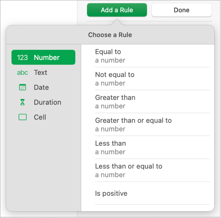
Click Conditional Highlighting, then click Add a Rule.
Click a type of rule (for example, if your cell value will be a number, select Numbers), then click a rule.
Scroll to see more options.

Enter values for the rule.
For example, if you selected the rule “date is after,” enter a date that the date in the cell must come after.
Click
 to use a cell reference. A cell reference lets you compare the cell’s value to another cell—so, for example, you can highlight a cell when its value is greater than another cell’s. Click a cell to select it, or enter its table address (for example, F1). See Calculate values using data in table cells in Numbers on Mac.
Click the pop-up menu and choose a text style, such as bold or italic, or a cell fill, such as red or green.
You can choose Custom Style to choose your own font color, font style, and cell fill.
Click Done.
Note: If a cell matches multiple rules, its look changes according to the first rule in the list. To reorder rules, drag the rule name up or down the list.
Repeat a highlighting rule
Delete a highlighting rule
Select cells with the rules you want to delete.
In the Format
 sidebar, click the Cell tab.
Click Show Highlighting Rules, then do one of the following:
Delete all rules for the selected cells: Click
 at the bottom of the sidebar, then choose Clear All Rules.
Delete a specific rule: Move the pointer over the rule, then click
 in the top-right corner.
Remove a rule from all cells that use it: Click
 at the bottom of the sidebar, choose Select Cells with Matching Rules, move your pointer over the rule, then click
  in the top-right corner.
