iBet uBet web content aggregator. Adding the entire web to your favor.


Link to original content: https://pubmed.ncbi.nlm.nih.gov/35502582
The Jurassic rise of squamates as supported by lepidosaur disparity and evolutionary rates - PubMed Skip to main page content
U.S. flag

An official website of the United States government

Dot gov

The .gov means it’s official.
Federal government websites often end in .gov or .mil. Before sharing sensitive information, make sure you’re on a federal government site.

Https

The site is secure.
The https:// ensures that you are connecting to the official website and that any information you provide is encrypted and transmitted securely.

Access keys NCBI Homepage MyNCBI Homepage Main Content Main Navigation
. 2022 May 3:11:e66511.
doi: 10.7554/eLife.66511.

The Jurassic rise of squamates as supported by lepidosaur disparity and evolutionary rates

Affiliations

The Jurassic rise of squamates as supported by lepidosaur disparity and evolutionary rates

Arnau Bolet et al. Elife. .

Abstract

The squamates (lizards, snakes, and relatives) today comprise more than 10,000 species, and yet their sister group, the Rhynchocephalia, is represented by a single species today, the tuatara. The explosion in squamate diversity has been tracked back to the Cretaceous Terrestrial Revolution, 100 million years ago (Ma), the time when flowering plants began their takeover of terrestrial ecosystems, associated with diversification of coevolving insects and insect-eating predators such as lizards, birds, and mammals. Squamates arose much earlier, but their long pre-Cretaceous history of some 150 million years (Myr) is documented by sparse fossils. Here, we provide evidence for an initial radiation of squamate morphology in the Middle and Late Jurassic (174-145 Ma), and show that they established their key ecological roles much earlier than had been assumed, and they have not changed them much since.

Keywords: Disparity; Lepidosauria; Macroevolution; Reptilia; Squamata; evolutionary biology; fossil record.


Conflict of interest statement

AB, TS, JH, MB No competing interests declared

Figures
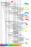
Figure 1.
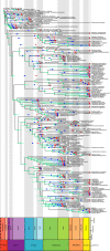
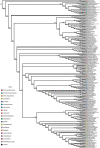
Figure 1.. Lepidosaur— phylogeny, morphospace, disparity, and evolutionary rates.
Phylogeny represented by a single randomly selected tree among those most parsimonious trees (MPTs) of the constrained analysis, and temporarily calibrated with the ‘Hedman’ method. Fossil ranges for each lineage are indicated according to the temporal distribution of the sampled taxa. For complete phylogenies and alternative datings, see Figure 1—figure supplements 1–7.
Figure 1—figure supplement 1.
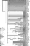
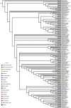
Figure 1—figure supplement 1.. Single, randomly selected, most parsimonious tree among those resulting from the constrained analysis of lepidosaurs, dated using the equal method, and showing the position and ranges of nodes times using all three methods (Hedman in green, equal in blue, and MBL in red).
Figure 1—figure supplement 2.
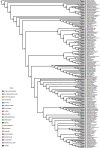
Figure 1—figure supplement 2.. Majority rule consensus tree for the constrained analysis of lepidosaurs.
Figure 1—figure supplement 3.
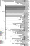
Figure 1—figure supplement 3.. Adams consensus tree for the constrained analysis of lepidosaurs.
Figure 1—figure supplement 4.
Figure 1—figure supplement 4.. Strict consensus tree for the constrained analysis of lepidosaurs.
Figure 1—figure supplement 5.
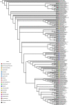
Figure 1—figure supplement 5.. Majority rule consensus tree for the unconstrained analysis of lepidosaurs.
Figure 1—figure supplement 6.
Figure 1—figure supplement 6.. Adams consensus tree for the unconstrained analysis of lepidosaurs.
Figure 1—figure supplement 7.
Figure 1—figure supplement 7.. Strict consensus tree for the unconstrained analysis of lepidosaurs.
Figure 2.
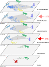
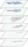
Figure 2.. Morphospace occupation through time.
Blue circles correspond to squamates, with the blue scincid silhouette indicating the position of generalized lizards, the yellow varanid indicating the position of anguimorphs, and the violet snake the position of snakes (and other limbless squamates). Green triangles correspond to rhynchocephalians (green Sphenodon silhouette). Red crosses correspond to stem lepidosaurs (red kuehneosaur silhouette). For additional plots of morphospace occupation through time, see Figure 2—figure supplements 1–6. JME: Jurassic Morphospace Expansion; KTR: Cretaceous Terrestrial Revolution.
Figure 2—figure supplement 1.
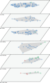
Figure 2—figure supplement 1.. Morphospace of lepidosaurs through time for PCO1 and PCO2.
Colors and symbols according to high-level taxonomical groups. Time bin ages correspond to time scheme 1.
Figure 2—figure supplement 2.
Figure 2—figure supplement 2.. Morphospace of lepidosaurs through time for PCO1 and PCO2.
Colors and symbols according to high-level taxonomical groups. Time bin ages correspond to time scheme 2.
Figure 2—figure supplement 3.
Figure 2—figure supplement 3.. Morphospace of lepidosaurs through time for PCO3 and PCO4.
Colors and symbols according to high-level taxonomical groups. Time bin ages correspond to time scheme 1.
Figure 2—figure supplement 4.
Figure 2—figure supplement 4.. Morphospace of lepidosaurs through time for PCO3 and PCO4.
Colors and symbols according to high-level taxonomical groups. Time bin ages correspond to time scheme 2.
Figure 2—figure supplement 5.
Figure 2—figure supplement 5.. Morphospace of lepidosaurs through time for PCO5 and PCO6.
Colors and symbols according to high-level taxonomical groups. Time bin ages correspond to time scheme 1.
Figure 2—figure supplement 6.
Figure 2—figure supplement 6.. Morphospace of lepidosaurs through time for PCO5 and PCO6.
Colors and simbols according to high-level taxonomical groups. Time bin ages correspond to time scheme 2.
Figure 3.
Figure 3.. Lepidosaur morphospace.
(A) Morphospace based on the two major axes of variation (PCO1 and PCO2), with colors and symbols according to the three main taxonomic groups. (B) Phylomorphospace distribution in PCO1 and PCO2, with lower taxonomic groups labeled. (C) 3D phylomorphospace illustrating the three major axes of variation (corresponding to PCO1, PCO2, and PCO3), with colors and symbols denoting to the lower taxonomic groups (see color legend in Figure 1—figure supplement 2). (D) Chronophylomorphospace of lepidosaurs showing the expansion of morphologies on the two major axes of variation (PCO1 and PCO2) through time. The phylogeny used corresponds to a randomly selected most parsimonious tree (MPT) of the constrained analysis. Silhouettes correspond to the same groups in Figure 1. JME: Jurassic Morphospace Expansion; KTR: Cretaceous Terrestrial Revolution. For additional plots of morphospace, see Figure 3—figure supplements 1–5, and Supplementary files 1-5.
Figure 3—figure supplement 1.
Figure 3—figure supplement 1.. Lepidosaur morphospace for PCO1 and PCO2 showing abbreviated taxa labels and colors according to clades (see color legend in Figure 1—figure supplement 2).
Abbreviations correspond to Ac plum: Acontias plumbeus; Ad magn: Adamisaurus magnidentatus; Ad sues: Adriosaurus suessi; Ae feli: Aeluroscalabotes felinus; Af aviu: Afairiguana avius; Ag agam: Agama agama; Ai: Aigialosaurus; Al fest: Alopoglossus festae; Am amei: Ameiva ameiva; An caro: Anolis carolinensis; An gilm: Anchaurosaurus gilmorei; An leon: Anomochilus leonardi; An pach: Ankylosphenodon pachyostosus; An papi: Anelytropsis papillosus; An scyt: Anilius scytale; Ar brev: Ardeosaurus brevipes; Ar orna: Arretosaurus ornatus; As tigr: Aspidoscelis tigris; Ba ammo: Bahndwivici ammoskius; Ba bico: Bachia bicolor; Ba macr: Bavarisaurus macrodactylus; Ba parv: Bainguis parvus; Be hoff: Becklesius hoffstetteri; Bi bipo: Bipes biporus; Bl: Blanus; Bo cons: Boa constrictor; Br: Brachylophus; Br bryg: Brookesia brygooi; Ca blan: Cadea blanoides; Ca drac: Callisaurus draconoides; Ca inte: Carusia intermedia; Ch fitz: Chometokadmon fitzingeri; Ch kozl: Cherminsaurus kozlowskii; Ch mada: Chalarodon madagascariensis; Ch ocel: Chalcides ocellatus; Cl bair: Clevosaurus bairdi; Cl bras: Clevosaurus brasiliensis; Cl mcgi: Clevosaurus mcgilli; Co mode: Colobosaura modesta; Cr coll: Crotaphytus collaris; Cr hass: Cryptolacerta hassiaca; Cr typi: Cricosaura typica; Ct parv: Ctenomastax parva; Cy huiz: Cynosphenodon huizachalensis; Cy ruff: Cylindrophis ruffus; Da este: Darchansaurus estesi; Da long: Dalinghosaurus longidigitus; Di avon: Diphydontosaurus avonis; Di nova: Dibamus novaeguineae; Di pata: Dinilysia patagonica; Do purb: Dorsetisaurus purbeckensis; Dr croi: Dracaenosaurus croizeti; Dr guia: Dracaena guianensis; Dr nord: Dryadosaura nordestina; Ei goul: Eichstaettisaurus gouldi; Ei schr: Eichstaettisaurus schroederi; El coer: Elgaria coerulea; En bili: Enyalius bilineatus; Eo koeh: Eosaniwa koehni; Eo lace: Eoxanta lacertifrons; Eo robu: Eolacerta robusta; Eo ster: Eonatator sternbergi; Ep goud: Epictia goudotii; Er robi: Erdenetesaurus robinsonae; Es mong: Estesia mongoliensis; Eu alge: Eumeces algeriensis; Eu macu: Eublepharis macularius; Ex serr: Exostinus serratus; Fe curr: Feylinia currori; Fl dzer: Flaviagama dzerzhinskii; Ga: Gambelia; Ge brid: Gephyrosaurus bridensis; Ge geck: Gekko gecko; Gi chul: Gilmoreteius chulsanensis; Gi ferr: Gilmoreteius ferrugenous; Gl semi: Gladidenagama semiplena; Gl venu: Globaura venusta; Go aren: Gobinatus arenosus; Go cret: Gobekko cretacicus; Go pulc: Gobiderma pulchrum; Gy unde: Gymnophthalmus underwoodi; Ha terr: Haasiophis terrasanctus; He horr: Heloderma horridum; Ho sanz: Hoyalacerta sanzi; Ho spin: Hoplocercus spinosus; Ho such: Hoburogekko suchanovi; Hu mixt: Huehuecuetzpalli mixtecus; Hy clar: Hymenosaurus clarki; Ic sief: Icarosaurus siefkeri; Ju gran: Jucaraseps grandipes; Ka ceri: Kallimodon cerinensis; Ku latu: Kuehneosaurus latus; La born: Lanthanotus borneensis; La serr: Laemanctus serratus; La viri: Lacerta viridis; Le cata: Leiosaurus catamarcensis; Le flav: Lepidophyma flavimaculatum; Li: Liolaemus; Li acan: Liushusaurus acanthocaudata; Li albi: Liotyphlops albirostris; Ly bowr: Lygosoma bowringii; Ma mabo: Mabuya mabouya; Ma oxon: Marmoretta oxoniensis; Me diaz: Meyasaurus diazromerali; Me orna: Merkurosaurus ornatus; Mi albe: Microlophus albermalensis; Mi cras: Mimeosaurus crassus; Mo annu: Morunasaurus annularis; Mo sund: Mochlus sundevalli; My micr: Myrmecodaptria microphagosa; Na rion: Najash rionegrina; Ne levi: Nephrurus levis; No nyct: Norellius nyctisaurops; Oe tryo: Oedura tryoni; Op cycl: Oplurus cyclurus; Or metz: Ornatocephalus metzleri; Pa UTAH: Paramacellodid UTAH; Pa angu: Paravaranus angustifrons; Pa bava: Palaeolacerta bavarica; Pa boge: Paraderma bogerti; Pa cana: Palaeosaniwa canadensis; Pa este: Parviraptor estesi; Pa inex: Parviderma inexacta; Pa kyre: Palaeoxantusia kyrentos; Pa owen: Paramacellodus oweni; Pa polo: Pamelina polonica; Pa posi: Palaeopleurosaurus posidoniae; Pa prob: Pachyrhachis problematicus; Pa scut: Parmeosaurus scutatus; Pa tlay: Pamizinsaurus tlayuaensis; Pa wyom: Parasaniwa wyomingensis; Pe gran: Peltosaurus granulosus; Ph asio: Phrynosoma asio; Ph aspe: Phrynosomimus asper; Ph coci: Physignathus cocincinus; Ph line: Phelsuma lineata; Pl anth: Plestiodon anthracinus; Pl fasc: Plestiodon fasciatus; Pl gold: Pleurosaurus goldfussi; Pl inte: Platysaurus intermedius; Pl plic: Plica plica; Pl robi: Planocephalosaurus robinsonae; Po ecpl: Potamites ecpleopus; Po gutt: Polychrus gutturosus; Po lign: Portugalophis lignites; Po mong: Polrussia mongoliensis; Po mull: Polysphenodon mulleri; Po ster: Polyglyphanodon sternbergi; Pr avel: Priosphenodon avelasi; Pr egge: Proscelotes eggeli; Pr gobi: Priscagama gobiensis; Pr long: Proplatynotia longirostrata; Pr ness: Primaderma nessovi; Ps beck: Pseudosaurillus becklesi; Ps gris: Psammosaurus griseus; Py lepi: Pygopus lepidopus; Re rugo: Restes rugosus; Rh flor: Rhineura floridana; Rh sang: Rhinophis sanguineus; Ri brac: Rieppeleon brachyurus; Sa ater: Sauromalus ater; Sa corn: Saltuarius cornutus; Sa davi: Saichangurvel davidsoni; Sa ensi: Saniwa ensidens; Sa feis: Saniwa feisti; Sa mong: Saniwides mongoliensis; Sc: Sceloporus; Sc cier: Scandensia ciervensis; Sc dysp: Schoenesmahl dyspepsia; Sc scin: Scincus scincus; Sh croc: Shinisaurus crocodilurus; Si hexa: Sineoamphisbaena hexatabularis; Sl dare: Slavoia darevskii; Sp eleg: Sphaerodactylus elegans; Sp punc: Sphenodon punctatus; St: Stenocercus; Ta sept: Takydromus septentrionalis; Tc mult: Tchingisaurus multivagus; Te elli: Temujinia ellisoni; Te gran: Telmasaurus grangeri; Te tepe: Tepexisaurus tepexii; Te teyo: Teius teyou; Ti scin: Tiliqua scincoides; Ti zhen: Tianyusaurus zhengi; Tr pete: Tracheloptychus petersi; Tr torq: Tropidurus torquatus; Tu tegu: Tupinambis teguixin; Ty grac: Typhlacontias gracilis; Ty jama: Typhlops jamaicensis; Ty squa: Typhlophis squamosus; Un gen PM: Unnamed gen PMUR58; Ur aegy: Uromastyx aegyptia; Ur nigr: Urosaurus nigricaudus; Ut stan: Uta stansburiana; Va vari: Varanus varius; Xa vigi: Xantusia vigilis; Xe gran: Xenosaurus grandis; Ya tenu: Yabeinosaurus tenuis; Za scel: Zapsosaurus sceliphros.
Figure 3—figure supplement 2.
Figure 3—figure supplement 2.. Lepidosaur morphospace for PCO3 and PCO4 showing abbreviated taxa labels and colors according to clades (see color legend in Figure 1—figure supplement 2 and abbreviations in Figure 3—figure supplement 1).
Figure 3—figure supplement 3.
Figure 3—figure supplement 3.. Lepidosaur morphospace for PCO5 and PCO6 showing abbreviated taxa labels and colors according to clades (see color legend in Figure 1—figure supplement 2 and abbreviations in Figure 3—figure supplement 1).
Figure 3—figure supplement 4.
Figure 3—figure supplement 4.. Lepidosaur morphospace for PCO1 and PCO2.
Colors, symbols, and hulls according to low-level taxonomical groups and colors according to clades (see color legend in Figure 1—figure supplement 2 and abbreviations in Figure 3—figure supplement 1).
Figure 3—figure supplement 5.
Figure 3—figure supplement 5.. Lepidosaur phylomorphospace in 2D for PCO1 and PCO2.
Colors according to high-level taxonomical groups and colors according to clades (see color legend in Figure 1—figure supplement 2 and abbreviations in Figure 3—figure supplement 1).
Figure 3—figure supplement 6.
Figure 3—figure supplement 6.. Plot of morphospace and clusters after applying the pamk function of the fpc package.
Clusters used in Figure 3B broadly correspond to the groups represented here and colors according to clades (see color legend in Figure 1—figure supplement 2 and abbreviations in Figure 3—figure supplement 1).
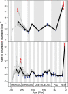
Figure 4.
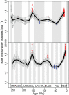
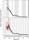
Figure 4.. Disparity and evolutionary rates through time.
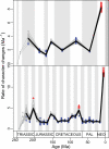
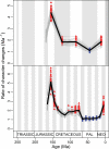
(A) Temporal disparity patterns (bootstrapped and rarefied within bin sum of variances for all axes). For additional plots of disparity patterns, see Figure 4—figure supplements 1–4. (B) Evolutionary rates through time in epoch-scale bins. Black solid line corresponds to results for all taxa, blue solid line for lizards, and green solid line for rhynchocephalians plus stem lepidosaurs (all according to the constrained phylogeny). Dashed gray line corresponds to results for all taxa and unconstrained phylogeny. The curves represent averages from 25 iterations of each analysis using randomly selected trees dated with the Hedman method. For additional plots of evolutionary rates, see Figure 4—figure supplements 5–22. JME: Jurassic Morphospace Expansion; KTR: Cretaceous Terrestrial Revolution; ETr: Early Triassic; MTr: Middle Triassic; LTr: Late Triassic; EJ: Early Jurassic; MJ: Middle Jurassic; LJ: Late Jurassic; EK: Early Cretaceous; LK: Late Cretaceous; Pg: Paleogene; Ng-Q: Neogene-Quaternary.
Figure 4—figure supplement 1.
Figure 4—figure supplement 1.. Disparity (weighted mean pairwise distance) by high taxonomical group.
Figure 4—figure supplement 2.
Figure 4—figure supplement 2.. Disparity (weighted mean pairwise distance) by low taxonomical group.
Figure 4—figure supplement 3.
Figure 4—figure supplement 3.. Disparity (weighted mean pairwise distance) through time for lepidosaurs and time scheme 1.
Figure 4—figure supplement 4.
Figure 4—figure supplement 4.. Disparity (weighted mean pairwise distance) through time for lepidosaurs and time scheme 2.
Figure 4—figure supplement 5.
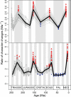
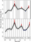
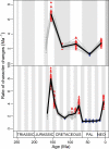
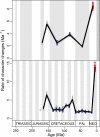
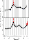
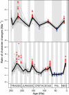
Figure 4—figure supplement 5.. Evolutionary rates for lepidosaurs according to the constrained phylogeny as represented by five most parsimonious trees (MPT) dated five times using the Hedman method.
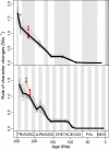
Spaghetti plot according to stratigraphic time bins (above); spaghetti plot according to 10 million year (Myr) time bins (below). Gray lines correspond to evolutionary rates for a specific dated MPT. Black line represents the average evolutionary rates. Red triangles and blue rhombuses highlight significantly high and significantly low evolutionary rates, respectively.
Figure 4—figure supplement 6.
Figure 4—figure supplement 6.. Evolutionary rates for lepidosaurs according to the constrained phylogeny as represented by five most parsimonious trees (MPTs) dated five times using the equal method.
Spaghetti plot according to stratigraphic time bins (above); spaghetti plot according to 10 million year (Myr) time bins (below). Gray lines correspond to evolutionary rates for a specific dated MPT. Black line represents the average evolutionary rates. Red triangles and blue rhombuses highlight significantly high and significantly low evolutionary rates, respectively.
Figure 4—figure supplement 7.
Figure 4—figure supplement 7.. Evolutionary rates for lepidosaurs according to the constrained phylogeny as represented by five most parsimonious trees (MPTs) dated five times using the MBL method.
Spaghetti plot according to stratigraphic time bins (above); spaghetti plot according to 10 million year (Myr) time bins (below). Gray lines correspond to evolutionary rates for a specific dated MPT. Black line represents the average evolutionary rates. Red triangles and blue rhombuses highlight significantly high and significantly low evolutionary rates, respectively.
Figure 4—figure supplement 8.
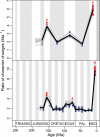
Figure 4—figure supplement 8.. Evolutionary rates for squamates according to the constrained phylogeny as represented by five most parsimonious trees (MPTs) dated five times using the Hedman method.
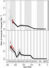
Spaghetti plot according to stratigraphic time bins (above); spaghetti plot according to 10 million year (Myr) time bins (below). Gray lines correspond to the average evolutionary rates. Red triangles and blue rhombuses highlight significantly high and significantly low evolutionary rates, respectively.
Figure 4—figure supplement 9.
Figure 4—figure supplement 9.. Evolutionary rates for squamates according to the constrained phylogeny as represented by five most parsimonious trees (MPTs) dated five times using the equal method.
Spaghetti plot according to stratigraphic time bins (above); spaghetti plot according to 10 million year (Myr) time bins (below). Gray lines correspond to evolutionary rates for a specific dated MPT. Black line represents the average evolutionary rates. Red triangles and blue rhombuses highlight significantly high and significantly low evolutionary rates, respectively.
Figure 4—figure supplement 10.
Figure 4—figure supplement 10.. Evolutionary rates for squamates according to the constrained phylogeny as represented by five most parsimonious trees (MPTs) dated five times using the MBL method.
Spaghetti plot according to stratigraphic time bins (above); spaghetti plot according to 10 million year (Myr) time bins (below). Gray lines correspond to evolutionary rates for a specific dated MPT. Black line represents the average evolutionary rates. Red triangles and blue rhombuses highlight significantly high and significantly low evolutionary rates, respectively.
Figure 4—figure supplement 11.
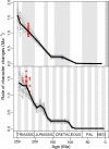
Figure 4—figure supplement 11.. Evolutionary rates for stem lepidosaurs plus rhynchocephalians according to the constrained phylogeny as represented by five most parsimonious trees (MPTs) dated five times using the Hedman method.
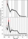
Spaghetti plot according to stratigraphic time bins (above); spaghetti plot according to 10 million year (Myr) time bins (below). Gray lines correspond to evolutionary rates for a specific dated MPT. Black line represents the average evolutionary rates. Red triangles and blue rhombuses highlight significantly high and significantly low evolutionary rates, respectively.
Figure 4—figure supplement 12.
Figure 4—figure supplement 12.. Evolutionary rates for stem lepidosaurs plus rhynchocephalians according to the constrained phylogeny as represented by five most parsimonious trees (MPTs) dated five times using the equal method.
Spaghetti plot according to stratigraphic time bins (above); spaghetti plot according to 10 million year (Myr) time bins (below). Gray lines correspond to evolutionary rates for a specific dated MPT. Black line represents the average evolutionary rates. Red triangles and blue rhombuses highlight significantly high and significantly low evolutionary rates, respectively.
Figure 4—figure supplement 13.
Figure 4—figure supplement 13.. Evolutionary rates for stem lepidosaurs plus rhynchocephalians according to the constrained phylogeny as represented by five most parsimonious trees (MPTs) dated five times using the MBL method.
Spaghetti plot according to stratigraphic time bins (above); spaghetti plot according to 10 million year (Myr) time bins (below). Gray lines correspond to evolutionary rates for a specific dated MPT. Black line represents the average evolutionary rates. Red triangles and blue rhombuses highlight significantly high and significantly low evolutionary rates, respectively.
Figure 4—figure supplement 14.
Figure 4—figure supplement 14.. Evolutionary rates for lepidosaurs according to the unconstrained phylogeny as represented by five most parsimonious trees (MPTs) dated five times using the Hedman method.
Spaghetti plot according to stratigraphic time bins (above); spaghetti plot according to 10 million year (Myr) time bins (below). Gray lines correspond to evolutionary rates for a specific dated MPT. Black line represents the average evolutionary rates. Red triangles and blue rhombuses highlight significantly high and significantly low evolutionary rates, respectively.
Figure 4—figure supplement 15.
Figure 4—figure supplement 15.. Evolutionary rates for lepidosaurs according to the unconstrained phylogeny as represented by five most parsimonious trees (MPTs) dated five times using the equal method.
Spaghetti plot according to stratigraphic time bins (above); spaghetti plot according to 10 million year (Myr) time bins (below). Gray lines correspond to evolutionary rates for a specific dated MPT. Black line represents the average evolutionary rates. Red triangles and blue rhombuses highlight significantly high and significantly low evolutionary rates, respectively.
Figure 4—figure supplement 16.
Figure 4—figure supplement 16.. Evolutionary rates for lepidosaurs according to the unconstrained phylogeny as represented by five most parsimonious trees (MPTs) dated five times using the MBL method.
Spaghetti plot according to stratigraphic time bins (above); spaghetti plot according to 10 million year (Myr) time bins (below). Gray lines correspond to evolutionary rates for a specific dated MPT. Black line represents the average evolutionary rates. Red triangles and blue rhombuses highlight significantly high and significantly low evolutionary rates, respectively.
Figure 4—figure supplement 17.
Figure 4—figure supplement 17.. Evolutionary rates for squamates according to the unconstrained phylogeny as represented by five most parsimonious trees (MPTs) dated five times using the Hedman method.
Spaghetti plot according to stratigraphic time bins (above); spaghetti plot according to 10 million year (Myr) time bins (below). Gray lines correspond to evolutionary rates for a specific dated MPT. Black line represents the average evolutionary rates. Red triangles and blue rhombuses highlight significantly high and significantly low evolutionary rates, respectively.
Figure 4—figure supplement 18.
Figure 4—figure supplement 18.. Evolutionary rates for squamates according to the unconstrained phylogeny as represented by five most parsimonious trees (MPTs) dated five times using the equal method.
Spaghetti plot according to stratigraphic time bins (above); spaghetti plot according to 10 million year (Myr) time bins (below). Gray lines correspond to evolutionary rates for a specific dated MPT. Black line represents the average evolutionary rates. Red triangles and blue rhombuses highlight significantly high and significantly low evolutionary rates, respectively.
Figure 4—figure supplement 19.
Figure 4—figure supplement 19.. Evolutionary rates for squamates according to the unconstrained phylogeny as represented by five most parsimonious trees (MPTs) dated five times using the MBL method.
Spaghetti plot according to stratigraphic time bins (above); spaghetti plot according to 10 million year (Myr) time bins (below). Gray lines correspond to evolutionary rates for a specific dated MPT. Black line represents the average evolutionary rates. Red triangles and blue rhombuses highlight significantly high and significantly low evolutionary rates, respectively.
Figure 4—figure supplement 20.
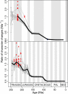
Figure 4—figure supplement 20.. Evolutionary rates for stem lepidosaurs and rhynchocephalians according to the unconstrained phylogeny as represented by five most parsimonious trees (MPTs) dated five times using the Hedman method.
Spaghetti plot according to stratigraphic time bins (above); spaghetti plot according to 10 million year (Myr) time bins (below). Gray lines correspond to evolutionary rates for a specific dated MPT. Black line represents the average evolutionary rates. Red triangles and blue rhombuses highlight significantly high and significantly low evolutionary rates, respectively.
Figure 4—figure supplement 21.
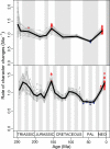
Figure 4—figure supplement 21.. Evolutionary rates for stem lepidosaurs and rhynchocephalians according to the unconstrained phylogeny as represented by five most parsimonious trees (MPTs) dated five times using the equal method.
(a) Spaghetti plot according to stratigraphic time bins; (b) spaghetti plot according to 10 million year (Myr) time bins. Gray lines correspond to evolutionary rates for a specific dated MPT. Black line represents the average evolutionary rates. Red triangles and blue rhombuses highlight significantly high and significantly low evolutionary rates, respectively.
Figure 4—figure supplement 22.
Figure 4—figure supplement 22.. Evolutionary rates for stem lepidosaurs and rhynchocephalians according to the unconstrained phylogeny as represented by five most parsimonious trees (MPTs) dated five times using the MBL method.
Spaghetti plot according to stratigraphic time bins (above); spaghetti plot according to 10 million year (Myr) time bins (below). Gray lines correspond to evolutionary rates for a specific dated MPT. Black line represents the average evolutionary rates. Red triangles and blue rhombuses highlight significantly high and significantly low evolutionary rates, respectively.
Appendix 1—figure 1.
Appendix 1—figure 1.. Completeness percentage by time bin for the complete dataset (all lepidosaurs and stem), for time scheme 1.
Appendix 1—figure 2.
Appendix 1—figure 2.. Completeness percentage by time bin for the complete dataset (all lepidosaurs and stem) for time scheme 2.
Appendix 1—figure 3.
Appendix 1—figure 3.. Completeness percentage by time bin for squamates and time scheme 1.
Appendix 1—figure 4.
Appendix 1—figure 4.. Completeness percentage by time bin for squamates and time scheme 2.
N/A
Appendix 1—figure 5.
Appendix 1—figure 5.. Plot of the number of taxa sampled for each time bin in (A) time scheme 1 and (B) time scheme 2.
Appendix 1—figure 6.
Appendix 1—figure 6.. Percentage of variance explained by each axis.
Appendix 1—figure 7.
Appendix 1—figure 7.. Plot of Cramér coefficients for PCO1 and PCO2 for the full dataset.
Characters do not appear in the original order because they have been grouped by anatomical regions. Inside each region, characters on the left are significant (according to their p-values, in green when significant, in red when not significant).
Appendix 2—figure 1.
Appendix 2—figure 1.. Morphospace (PCO1 and PCO2) when myological/integument (except for osteoderm characters) are deactivated.
Appendix 2—figure 2.
Appendix 2—figure 2.. Plot of Cramér coefficients for PCO1 and PCO2 for the dataset without myological/integument (except for osteoderm characters), limited to characters with a coefficient <0.4.
Character numbers correspond to those of the original morphological matrix. Significant characters are marked with an asterisk.
Appendix 3—figure 1.
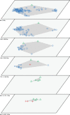
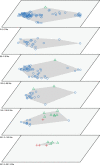
Appendix 3—figure 1.. Chronophylomorphospace for squamates.
Screenshot of the interactive plot in two (A, B) views. Colors correspond to low-level taxonomical groups. The solid red arrow points to the morphospace expansion occurring by the Middle–Late Jurassic, and the light red arrow to a minor event occurring around the middle–Late Cretaceous boundary.
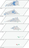
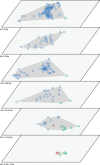
Appendix 3—figure 2.
Appendix 3—figure 2.. Phylomorphospace in 3D for PCO1, PCO2, and PCO3 for squamates only.
Screenshot of the interactive plot, where black spheres correspond to toxicoferan squamates and white spheres correspond to non-toxicoferan squamates.
Similar articles

Cited by

References

    1. Adams D, Collyer M, Kaliontzopoulou A. geomorph: an r package for the collection and analysis of geometric morphometric shape data. Methods in Ecology and Evolution. 2019;1:12035. doi: 10.1111/2041-210X.12035. - DOI
    1. Bapst DW. Paleotree: an R package for paleontological and phylogenetic analyses of evolution. Methods in Ecology and Evolution. 2012;3:803–807. doi: 10.1111/j.2041-210X.2012.00223.x. - DOI
    1. Benson RBJ, Campione NE, Carrano MT, Mannion PD, Sullivan C, Upchurch P, Evans DC. Rates of dinosaur body mass evolution indicate 170 million years of sustained ecological innovation on the avian stem lineage. PLOS Biology. 2014;12:e1001853. doi: 10.1371/journal.pbio.1001853. - DOI - PMC - PubMed
    1. Benton MJ. The origins of modern biodiversity on land. Philosophical Transactions of the Royal Society of London. Series B, Biological Sciences. 2010;365:3667–3679. doi: 10.1098/rstb.2010.0269. - DOI - PMC - PubMed
    1. Bolet A, Evans SE. New material of the enigmatic Scandensia, an Early Cretaceous lizard from the Iberian Peninsula. Spec. Pap. Palaeontol. 2011;86:99–108. doi: 10.1111/J.1475-4983.2011.01074.x. - DOI

Publication types

Grants and funding

The funders had no role in study design, data collection and interpretation, or the decision to submit the work for publication.