Abstract
Kernel smoother and a time-histogram are classical tools for estimating an instantaneous rate of spike occurrences. We recently established a method for selecting the bin width of the time-histogram, based on the principle of minimizing the mean integrated square error (MISE) between the estimated rate and unknown underlying rate. Here we apply the same optimization principle to the kernel density estimation in selecting the width or “bandwidth” of the kernel, and further extend the algorithm to allow a variable bandwidth, in conformity with data. The variable kernel has the potential to accurately grasp non-stationary phenomena, such as abrupt changes in the firing rate, which we often encounter in neuroscience. In order to avoid possible overfitting that may take place due to excessive freedom, we introduced a stiffness constant for bandwidth variability. Our method automatically adjusts the stiffness constant, thereby adapting to the entire set of spike data. It is revealed that the classical kernel smoother may exhibit goodness-of-fit comparable to, or even better than, that of modern sophisticated rate estimation methods, provided that the bandwidth is selected properly for a given set of spike data, according to the optimization methods presented here.
Keywords: Kernel density estimation, Bandwidth optimization, Mean integrated squared error
Introduction
Neurophysiologists often investigate responses of a single neuron to a stimulus presented to an animal by using the discharge rate of action potentials, or spikes (Adrian 1928; Gerstein and Kiang 1960; Abeles 1982). One classical method for estimating spike rate is the kernel density estimation (Parzen 1962; Rosenblatt 1956; Sanderson 1980; Richmond et al. 1990; Nawrot et al. 1999). In this method, a spike sequence is convoluted with a kernel function, such as a Gauss density function, to obtain a smooth estimate of the firing rate. The estimated rate is sometimes referred to as a spike density function. This nonparametric method is left with a free parameter for kernel bandwidth that determines the goodness-of-fit of the density estimate to the unknown rate underlying data. Although theories have been suggested for selecting the bandwidth, cross-validating with the data (Rudemo 1982; Bowman 1984; Silverman 1986; Scott and Terrell 1987; Scott 1992; Jones et al. 1996; Loader 1999a, b), individual researchers have mostly chosen bandwidth arbitrarily. This is partly because the theories have not spread to the neurophysiological society, and partly due to inappropriate basic assumptions of the theories themselves. Most optimization methods assume a stationary rate fluctuation, while the neuronal firing rate often exhibits abrupt changes, to which neurophysiologists, in particular, pay attention. A fixed bandwidth, optimized using a stationary assumption, is too wide to extract the details of sharp activation, while in the silent period, the fixed bandwidth would be too narrow and may cause spurious undulation in the estimated rate. It is therefore desirable to allow a variable bandwidth, in conformity with data.
The idea of optimizing bandwidth at every instant was proposed by Loftsgaarden and Quesenberry (1965). However, in contrast to the progress in methods that vary bandwidths at sample points only (Abramson 1982; Breiman et al. 1977; Sain and Scott 1996; Sain 2002; Brewer 2004), the local optimization of bandwidth at every instant turned out to be difficult because of its excessive freedom (Scott 1992; Devroye and Lugosi 2000; Sain and Scott 2002). In earlier studies, Hall & Schucany used the cross-validation of Rudemo and Bowman, within local intervals (Hall and Schucany 1989), yet the interval length was left free. Fan et al. applied cross-validation to locally optimized bandwidth (Fan et al. 1996), and yet the smoothness of the variable bandwidth was chosen manually.
In this study, we first revisit the fixed kernel method, and derive a simple formula to select the bandwidth of the kernel density estimation, similar to the previous method for selecting the bin width of a peristimulus time histogram (See Shimazaki and Shinomoto 2007). Next, we introduce the variable bandwidth into the kernel method and derive an algorithm for determining the bandwidth locally in time. The method automatically adjusts the flexibility, or the stiffness, of the variable bandwidth. The performance of our fixed and variable kernel methods are compared with established density estimation methods, in terms of the goodness-of-fit to underlying rates that vary either continuously or discontinuously. We also apply our kernel methods to the biological data, and examine their ability by cross-validating with data.
Though our methods are based on the classical kernel method, their performances are comparable to various sophisticated rate estimation methods. Because of the classics, they are rather convenient for users: the methods simply suggest bandwidth for the standard kernel density estimation.
Methods
Kernel smoothing
In neurophysiological experiments, neuronal response is examined by repeatedly applying identical stimuli. The recorded spike trains are aligned at the onset of stimuli, and superimposed to form a raw density, as
 |
1 |
where n is the number of repeated trials. Here, each spike is regarded as a point event that occurs at an instant of time t i (i = 1,2, ⋯ , N) and is represented by the Dirac delta function δ(t). The kernel density estimate is obtained by convoluting a kernel k(s) to the raw density x t,
 |
2 |
Throughout this study, the integral  that does not specify bounds refers to
  . The kernel function satisfies the normalization condition,
  , a zero first moment,
  , and has a finite bandwidth,
  . A frequently used kernel is the Gauss density function,
 |
3 |
where the bandwidth w is specified as a subscript. In the body of this study, we develop optimization methods that apply generally to any kernel function, and derive a specific algorithm for the Gauss density function in the Appendix.
Mean integrated squared error optimization principle
Assuming that spikes are sampled from a stochastic process, we consider optimizing the estimate  to be closest to the unknown underlying rate λ
t. Among several plausible optimizing principles, such as the Kullback-Leibler divergence or the Hellinger distance, we adopt, here, the mean integrated squared error (MISE) for measuring the goodness-of-fit of an estimate to the unknown underlying rate, as
 |
4 |
where E refers to the expectation with respect to the spike generation process under a given inhomogeneous rate λ t. It follows, by definition, that Ex t = λ t.
In deriving optimization methods, we assume the Poisson nature, so that spikes are randomly sampled at a given rate λ
t. Spikes recorded from a single neuron correlate in each sequence (Shinomoto et al. 2003, 2005, 2009). In the limit of a large number of spike trains, however, mixed spikes are statistically independent and the superimposed sequence can be approximated as a single inhomogeneous Poisson point process (Cox 1962; Snyder 1975; Daley and Vere-Jones 1988; Kass et al. 2005).
Selection of the fixed bandwidth
Given a kernel function such as Eq. (3), the density function Eq. (2) is uniquely determined for a raw density Eq. (1) of spikes obtained from an experiment. A bandwidth w of the kernel may alter the density estimate, and it can accordingly affect the goodness-of-fit of the density function  to the unknown underlying rate λ
t. In this subsection, we consider applying a kernel of a fixed bandwidth w, and develop a method for selecting w that minimizes the MISE, Eq. (4).
The integrand of the MISE is decomposed into three parts:  . Since the last component does not depend on the choice of a kernel, we subtract it from the MISE, then define a cost function as a function of the bandwidth w:
 |
5 |
Rudemo and Bowman suggested the leave-one-out cross-validation to estimate the second term of Eq. (5) (Rudemo 1982; Bowman 1984). Here, we directly estimate the second term with the Poisson assumption (See also Shimazaki and Shinomoto 2007).
By noting that λ t = Ex t, the integrand of the second term in Eq. (5) is given as
 |
6 |
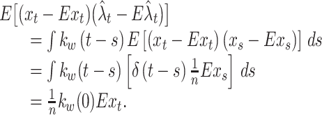
from a general decomposition of covariance of two random variables. Using Eq. (2), the covariance (the second term of Eq. (6)) is obtained as
 |
7 |
Here, to obtain the second equality, we used the assumption of the Poisson point process (independent spikes).
Using Eqs. (6) and (7), Eq. (5) becomes
 |
8 |
Equation (8) is composed of observable variables only. Hence, from sample sequences, the cost function is estimated as
 |
9 |
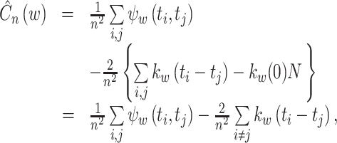
In terms of a kernel function, the cost function is written as
 |
10 |
where
 |
11 |
The minimizer of the cost function, Eq. (10), is an estimate of the optimal bandwidth, which is denoted by w
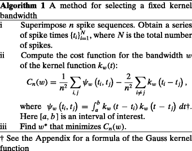
∗ . The method for selecting a fixed kernel bandwidth is summarized in Algorithm 1. A particular algorithm developed for the Gauss density function is given in the Appendix.

Selection of the variable bandwidth
The method described in Section 2.3 aims to select a single bandwidth that optimizes the goodness-of-fit of the rate estimate for an entire observation interval [a, b] . For a non-stationary case, in which the degree of rate fluctuation greatly varies in time, the rate estimation may be improved by using a kernel function whose bandwidth is adaptively selected in conformity with data. The spike rate estimated with the variable bandwidth w t is given by
 |
12 |
Here we select the variable bandwidth w t as a fixed bandwidth optimized in a local interval. In this approach, the interval length for the local optimization regulates the shape of the function w t, therefore, it subsequently determines the goodness-of-fit of the estimated rate to the underlying rate. We provide a method for obtaining the variable bandwidth w t that minimizes the MISE by optimizing the local interval length.
To select an interval length for local optimization, we introduce the local MISE criterion at time t as
 |
13 |
where  is an estimated rate with a fixed bandwidth w. Here, a weight function
  localizes the integration of the squared error in a characteristic interval W centered at time t. An example of the weight function is once again the Gauss density function. See the Appendix for the specific algorithm for the Gauss weight function. As in Eq. (5), we introduce the local cost function at time t by subtracting the term irrelevant for the choice of w as
 |
14 |
The optimal fixed bandwidth w ∗ is obtained as a minimizer of the estimated cost function:
 |
15 |
where
 |
16 |
The derivation follows the same steps as in the previous section. Depending on the interval length W, the optimal bandwidth w
∗ varies. We suggest selecting an interval length that scales with the optimal bandwidth as γ
− 1
w
∗ . The parameter γ regulates the interval length for local optimization: With small γ( ≪ 1) , the fixed bandwidth is optimized within a long interval; With large γ(~1) , the fixed bandwidth is optimized within a short interval. The interval length and fixed bandwidth, selected at time t, are denoted as  and
and  .
.
The locally optimized bandwidth  is repeatedly obtained for different t( ∈ [a,b]). Because the intervals overlap, we adopt the Nadaraya-Watson kernel regression (Nadaraya 1964; Watson 1964) of
  as a local bandwidth at time t:
 |
17 |
The variable bandwidth  obtained from the same data, but with different γ, exhibits different degrees of smoothness: With small γ( ≪ 1) , the variable bandwidth fluctuates slightly; With large γ(~1) , the variable bandwidth fluctuates significantly. The parameter γ is thus a smoothing parameter for the variable bandwidth. Similar to the fixed bandwidth, the goodness-of-fit of the variable bandwidth can be estimated from the data. The cost function for the variable bandwidth selected with γ is obtained as
 |
18 |
where  is an estimated rate, with the variable bandwidth
  . The integral is calculated numerically. With the stiffness constant γ
∗ that minimizes Eq. (18), local optimization is performed in an ideal interval length. The method for optimizing the variable kernel bandwidth is summarized in Algorithm 2.
Results
Comparison of the fixed and variable kernel methods
By using spikes sampled from an inhomogeneous Poisson point process, we examined the efficiency of the kernel methods in estimating the underlying rate. We also used a sequence obtained by superimposing ten non-Poissonian (gamma) sequences (Shimokawa and Shinomoto 2009), but there was practically no significant difference in the rate estimation from the Poissonian sequence.
Figure 1 displays the result of the fixed kernel method based on the Gauss density function. The kernel bandwidth selected by Algorithm 1 applies a reasonable filtering to the set of spike sequences. Figure 1(d) shows that a cost function, Eq. (10), estimated from the spike data is similar to the original MISE, Eq. (4), which was computed using the knowledge of the underlying rate. This demonstrates that MISE optimization can, in practice, be carried out by our method, even without knowing the underlying rate.
Fig. 1.
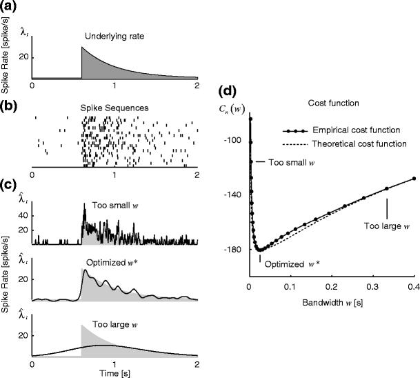
Fixed kernel density estimation. (a) The underlying spike rate λ t of the Poisson point process. (b) 20 spike sequences sampled from the underlying rate, and (c) Kernel rate estimates made with three types of bandwidth: too small, optimal, and too large. The gray area indicates the underlying spike rate. (d) The cost function for bandwidth w. Solid line is the estimated cost function, Eq. (10), computed from the spike data; The dashed line is the exact cost function, Eq. (5), directly computed by using the known underlying rate
Figure 2(a) demonstrates how the rate estimation is altered by replacing the fixed kernel method with the variable kernel method (Algorithm 2), for identical spike data (Fig. 1(b)). The Gauss weight function is used to obtain a smooth variable bandwidth. The manner in which the optimized bandwidth varies in the time axis is shown in Fig. 2(b): the bandwidth is short in a moment of sharp activation, and is long in the period of smooth rate modulation. Eventually, the sharp activation is grasped minutely and slow modulation is expressed without spurious fluctuations. The stiffness constant γ for the bandwidth variation is selected by minimizing the cost function, as shown in Fig. 2(c).
Fig. 2.
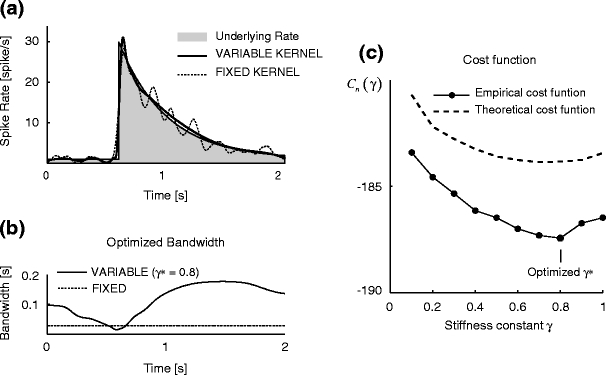
Variable kernel density estimation. (a) Kernel rate estimates. The solid and dashed lines are rate estimates made by the variable and fixed kernel methods for the spike data of Fig. 1(b). The gray area is the underlying rate. (b) Optimized bandwidths. The solid line is the variable bandwidth determined with the optimized stiffness constant γ ∗ = 0.8, selected by Algorithm 2; the dashed line is the fixed bandwidth selected by Algorithm 1. (b) The cost function for bandwidth stiffness constant. The solid line is the cost function for the bandwidth stiffness constant γ, Eq. (18), estimated from the spike data; the dashed line is the cost function computed from the known underlying rate
Comparison with established density estimation methods
We wish to examine the fitting performance of the fixed and variable kernel methods in comparison with established density estimation methods, by paying attention to their aptitudes for either continuous or discontinuous rate processes. Figure 3(a) shows the results for sinusoidal and sawtooth rate processes, as samples of continuous and discontinuous processes, respectively. We also examined triangular and rectangular rate processes as different samples of continuous and discontinuous processes, but the results were similar. The goodness-of-fit of the density estimate to the underlying rate is evaluated in terms of integrated squared error (ISE) between them.
Fig. 3.
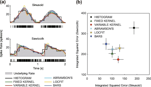
Fitting performances of the six rate estimation methods, histogram, fixed kernel, variable kernel, Abramson’s adaptive kernel, Locfit, and Bayesian adaptive regression splines (BARS). (a) Two rate profiles (2 [s]) used in generating spikes (gray area), and the estimated rates using six different methods. The raster plot in each panel is sample spike data (n = 10, superimposed). (b) Comparison of the six rate estimation methods in their goodness-of-fit, based on the integrated squared error (ISE) between the underlying and estimated rate. The abscissa and the ordinate are the ISEs of each method applied to sinusoidal and sawtooth underlying rates (10 [s]). The mean and standard deviation of performance evaluated using 20 data sets are plotted for each method
The established density estimation methods examined for comparison are the histogram (Shimazaki and Shinomoto 2007), Abramson’s adaptive kernel (Abramson 1982), Locfit (Loader 1999b), and Bayesian adaptive regression splines (BARS) (DiMatteo et al. 2001; Kass et al. 2003) methods, whose details are summarized below.
A histogram method, which is often called a peristimulus time histogram (PSTH) in neurophysiological literature, is the most basic method for estimating the spike rate. To optimize the histogram, we used a method proposed for selecting the bin width based on the MISE principle (Shimazaki and Shinomoto 2007).
Abramson’s adaptive kernel method (Abramson 1982) uses the sample point kernel estimate  , in which the bandwidths are adapted at the sample points. Scaling the bandwidths as
  was suggested, where w is a pilot bandwidth,
  , and
, and  is a fixed kernel estimate with w. Abramson’s method is a two-stage method, in which the pilot bandwidth needs to be selected beforehand. Here, the pilot bandwidth is selected using the fixed kernel optimization method developed in this study.
The Locfit algorithm developed by Loader (1999b) fits a polynomial to a log-density function under the principle of maximizing a locally defined likelihood. We examined the automatic choice of the adaptive bandwidth of the local likelihood, and found that the default fixed method yielded a significantly better fit. We used a nearest neighbor based bandwidth method, with a parameter covering 20% of the data.
The BARS (DiMatteo et al. 2001; Kass et al. 2003) is a spline-based adaptive regression method on an exponential family response model, including a Poisson count distribution. The rate estimated with the BARS is the expected splines computed from the posterior distribution on the knot number and locations with a Markov chain Monte Carlo method. The BARS is, thus, capable of smoothing a noisy histogram without missing abrupt changes. To create an initial histogram, we used 4 [ms] bin width, which is small enough to examine rapid changes in the firing rate.
Figure 3(a) displays the density profiles of the six different methods estimated from an identical set of spike trains (n = 10) that are numerically sampled from a sinusoidal or sawtooth underlying rate (2 [s]). Figure 3(b) summarizes the goodness-of-fit of the six methods to the sinusoidal and sawtooth rates (10 [s]) by averaging over 20 realizations of samples.
For the sinusoidal rate function, representing continuously varying rate processes, the BARS is most efficient in terms of ISE performance. For the sawtooth rate function, representing discontinuous non-stationary rate processes, the variable kernel estimation developed here is the most efficient in grasping abrupt rate changes. The histogram method is always inferior to the other five methods in terms of ISE performance, due to the jagged nature of the piecewise constant function.
Application to experimental data
We examine, here, the fixed and variable kernel methods in their applicability to real biological data. In particular, the kernel methods are applied to the spike data of an MT neuron responding to a random dot stimulus (Britten et al. 2004). The rates estimated from n = 1, 10, and 30 experimental trials are shown in Fig. 4. Fine details of rate modulation are revealed as we increase the sample size (Bair and Koch 1996). The fixed kernel method tends to choose narrower bandwidths, while the variable kernel method tends to choose wider bandwidths in the periods in which spikes are not abundant.
Fig. 4.
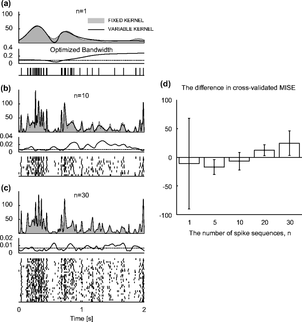
Application of the fixed and variable kernel methods to spike data of an MT neuron (j024 with coherence 51.2% in nsa2004.1 (Britten et al. 2004)). (a–c): Analyses of n = 1, 10, and 30 spike trains; (top) Spike rates [spikes/s] estimated with the fixed and variable kernel methods are represented by the gray area and solid line, respectively; (middle) optimized fixed and variable bandwidths [s] are represented by dashed and solid lines, respectively; (bottom) A raster plot of the spike data used in the estimation. (d) Comparison of the two kernel methods. Bars represent the difference between the cross-validated cost functions, Eq. (19), of the fixed and variable kernel methods (fix less variable). The positive difference indicates superior fitting performance of the variable kernel method. The cross-validated cost function is obtained as follows. Whole spike sequences ( ) are divided into
  blocks, each composed of n ( = 1, 5, 20, 30) spike sequences. A bandwidth was selected using spike data of a training block. The cross-validated cost functions, Eq. (19), for the selected bandwidth are computed using the
  leftover test blocks, and their average is computed. The cost function is repeatedly obtained
  -times by changing the training block. The mean and standard deviation, computed from
  samples, are displayed
The performance of the rate estimation methods is cross-validated. The bandwidth, denoted as w t for both fixed and variable, is obtained with a training data set of n trials. The error is evaluated by computing the cost function, Eq. (18), in a cross-validatory manner:
 |
19 |
where the test spike times  are obtained from n spike sequences in the leftovers, and
  . Figure 4(d) shows the performance improvements by the variable bandwidth over the fixed bandwidth, as evaluated by Eq. (19). The fixed and variable kernel methods perform better for smaller and larger sizes of data, respectively. In addition, we compared the fixed kernel method and the BARS by cross-validating the log-likelihood of a Poisson process with the rate estimated using the two methods. The difference in the log-likelihoods was not statistically significant for small samples (n = 1, 5 and 10), while the fixed kernel method fitted better to the spike data with larger samples (n = 20 and 30).
Discussion
In this study, we developed methods for selecting the kernel bandwidth in the spike rate estimation based on the MISE minimization principle. In addition to the principle of optimizing a fixed bandwidth, we further considered selecting the bandwidth locally in time, assuming a non-stationary rate modulation.
We tested the efficiency of our methods using spike sequences numerically sampled from a given rate (Figs. 1 and 2). Various density estimators constructed on different optimization principles were compared in their goodness-of-fit to the underlying rate (Fig. 3). There is in fact no oracle that selects one among various optimization principles, such as MISE minimization or likelihood maximization. Practically, reasonable principles render similar detectability for rate modulation; the kernel methods based on MISE were roughly comparable to the Locfit based on likelihood maximization in their performances. The difference of the performances is not due to the choice of principles, but rather due to techniques; kernel and histogram methods lead to completely different results under the same MISE minimization principle (Fig. 3(b)). Among the smooth rate estimators, the BARS was good at representing continuously varying rate, while the variable kernel method was good at grasping abrupt changes in the rate process (Fig. 3(b)).
We also examined the performance of our methods in application to neuronal spike sequences by cross-validating with the data (Fig. 4). The result demonstrated that the fixed kernel method performed well in small samples. We refer to Cunningham et al. (2008) for a result on the superior fitting performance of a fixed kernel to small samples in comparison with the Locfit and BARS, as well as the Gaussian process smoother (Cunningham et al. 2008; Smith and Brown 2003; Koyama and Shinomoto 2005). The adaptive methods, however, have the potential to outperform the fixed method with larger samples derived from a non-stationary rate profile (See also Endres et al. 2008 for comparisons of their adaptive histogram with the fixed histogram and kernel method). The result in Fig. 4 confirmed the utility of our variable kernel method for larger samples of neuronal spikes.
We derived the optimization methods under the Poisson assumption, so that spikes are randomly drawn from a given rate. If one wishes to estimate spike rate of a single or a few sequences that contain strongly correlated spikes, it is desirable to utilize the information as to non-Poisson nature of a spike train (Cunningham et al. 2008). Note that a non-Poisson spike train may be dually interpreted, as being derived either irregularly from a constant rate, or regularly from a fluctuating rate (Koyama and Shinomoto 2005; Shinomoto and Koyama 2007). However, a sequence obtained by superimposing many spike trains is approximated as a Poisson process (Cox 1962; Snyder 1975; Daley and Vere-Jones 1988; Kass et al. 2005), for which dual interpretation does not occur. Thus the kernel methods developed in this paper are valid for the superimposed sequence, and serve as the peristimulus density estimator for spike trains aligned at the onset or offset of the stimulus.
Kernel smoother is a classical method for estimating the firing rate, as popular as the histogram method. We have shown in this paper that the classical kernel methods perform well in the goodness-of-fit to the underlying rate. They are not only superior to the histogram method, but also comparable to modern sophisticated methods, such as the Locfit and BARS. In particular, the variable kernel method outperformed competing methods in representing abrupt changes in the spike rate, which we often encounter in neuroscience. Given simplicity and familiarity, the kernel smoother can still be the most useful in analyzing the spike data, provided that the bandwidth is chosen appropriately as instructed in this paper.
Acknowledgements
We thank M. Nawrot, S. Koyama, D. Endres for valuable discussions, and the Diesmann Unit for providing the computing environment. We also acknowledge K. H. Britten, M. N. Shadlen, W. T. Newsome, and J. A. Movshon, who made their data available to the public, and W. Bair for hosting the Neural Signal Archive. This study is supported in part by a Research Fellowship of the Japan Society for the Promotion of Science for Young Scientists to HS and Grants-in-Aid for Scientific Research to SS from the MEXT Japan (20300083, 20020012).
Open Access
This article is distributed under the terms of the Creative Commons Attribution Noncommercial License which permits any noncommercial use, distribution, and reproduction in any medium, provided the original author(s) and source are credited.
Appendix: Cost functions of the Gauss kernel function
In this appendix, we derive definite MISE optimization algorithms we developed in the body of the paper with the particular Gauss density function, Eq. (3).
A.1 A cost function for a fixed bandwidth
The estimated cost function is obtained, as in Eq. (10):
 |
where, from Eq. (11),
 |
A symmetric kernel function, including the Gauss function, is invariant to exchange of t i and t j when computing k w(t i − t j) . In addition, the correlation of the kernel function, Eq. (11), is symmetric with respect to t i and t j. Hence, we obtain the following relationships
 |
20 |
 |
21 |
By plugging Eqs. (20) and (21) into Eq. (10), the cost function is simplified as.
 |
22 |
For the Gauss kernel function, Eq. (3), with bandwidth w, Eq. (11) becomes
 |
23 |
where  . A simplified equation is obtained by evaluating the MISE in an unbounded domain: a→ − ∞ and b→ + ∞. Using
  , we obtain
 |
24 |
Using Eq. (24) in Eq. (22), we obtain a formula for selecting the bandwidth of the Gauss kernel function,  :
:
 |
25 |
A.2 A local cost function for a variable bandwidth
The local cost function is obtained, as in Eq. (15):
 |
where, from Eq. (16),
 |
For the summations in the local cost function, Eq. (15), we have equalities:
 |
26 |
 |
27 |
The first equation holds for a symmetric kernel. The second equation is derived because Eq. (16) is invariant to an exchange of t i and t j. Using Eqs. (26) and (27), Eq. (15) can be computed as
 |
28 |
For the Gauss kernel function and the Gauss weight function with bandwidth w and W respectively, Eq. (16) is calculated as
 |
29 |
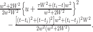
By completing the square with respect to u, the exponent in the above equation is written as
 |
30 |
Using the formula  , Eq. (16) is obtained as
 |
31 |
Contributor Information
Hideaki Shimazaki, Email: shimazaki@brain.riken.jp.
Shigeru Shinomoto, Email: shinomoto@scphys.kyoto-u.ac.jp.
References
- Abeles M. Quantification, smoothing, and confidence-limits for single-units histograms. Journal of Neuroscience Methods. 1982;5(4):317–325. doi: 10.1016/0165-0270(82)90002-4. [DOI] [PubMed] [Google Scholar]
- Abramson I. On bandwidth variation in kernel estimates-a square root law. The Annals of Statistics. 1982;10(4):1217–1223. doi: 10.1214/aos/1176345986. [DOI] [Google Scholar]
- Adrian E. The basis of sensation: The action of the sense organs. New York: W.W. Norton; 1928. [Google Scholar]
- Bair W, Koch C. Temporal precision of spike trains in extrastriate cortex of the behaving macaque monkey. Neural Computation. 1996;8(6):1185–1202. doi: 10.1162/neco.1996.8.6.1185. [DOI] [PubMed] [Google Scholar]
- Bowman AW. An alternative method of cross-validation for the smoothing of density estimates. Biometrika. 1984;71(2):353. doi: 10.1093/biomet/71.2.353. [DOI] [Google Scholar]
- Breiman L, Meisel W, Purcell E. Variable kernel estimates of multivariate densities. Technometrics. 1977;19:135–144. doi: 10.2307/1268623. [DOI] [Google Scholar]
- Brewer MJ. A Bayesian model for local smoothing in kernel density estimation. Statistics and Computing. 2004;10:299–309. doi: 10.1023/A:1008925425102. [DOI] [Google Scholar]
- Britten, K. H., Shadlen, M. N., Newsome, W. T., & Movshon, J. A. (2004). Responses of single neurons in macaque mt/v5 as a function of motion coherence in stochastic dot stimuli. The Neural Signal Archive. nsa2004.1. http://www.neuralsignal.org.
- Cox RD. Renewal theory. London: Wiley; 1962. [Google Scholar]
- Cunningham J, Yu B, Shenoy K, Sahani M, Platt J, Koller D, et al. Inferring neural firing rates from spike trains using Gaussian processes. Advances in Neural Information Processing Systems. 2008;20:329–336. [Google Scholar]
- Daley D, Vere-Jones D. An introduction to the theory of point processes. New York: Springer; 1988. [Google Scholar]
- Devroye L, Lugosi G. Variable kernel estimates: On the impossibility of tuning the parameters. In: Giné E, Mason D, Wellner JA, editors. High dimensional probability II. Boston: Birkhauser; 2000. pp. 405–442. [Google Scholar]
- DiMatteo I, Genovese CR, Kass RE. Bayesian curve-fitting with free-knot splines. Biometrika. 2001;88(4):1055–1071. doi: 10.1093/biomet/88.4.1055. [DOI] [Google Scholar]
- Endres D, Oram M, Schindelin J, Foldiak P. Bayesian binning beats approximate alternatives: Estimating peristimulus time histograms. Advances in Neural Information Processing Systems. 2008;20:393–400. [Google Scholar]
- Fan J, Hall P, Martin MA, Patil P. On local smoothing of nonparametric curve estimators. Journal of the American Statistical Association. 1996;91:258–266. doi: 10.2307/2291403. [DOI] [Google Scholar]
- Gerstein GL, Kiang NYS. An approach to the quantitative analysis of electrophysiological data from single neurons. Biophysical Journal. 1960;1(1):15–28. doi: 10.1016/S0006-3495(60)86872-5. [DOI] [PMC free article] [PubMed] [Google Scholar]
- Hall P, Schucany WR. A local cross-validation algorithm. Statistics & Probability Letters. 1989;8(2):109–117. doi: 10.1016/0167-7152(89)90002-3. [DOI] [Google Scholar]
- Jones M, Marron J, Sheather S. A brief survey of bandwidth selection for density estimation. Journal of the American Statistical Association. 1996;91(433):401–407. doi: 10.2307/2291420. [DOI] [Google Scholar]
- Kass RE, Ventura V, Brown EN. Statistical issues in the analysis of neuronal data. Journal of Neurophysiology. 2005;94(1):8–25. doi: 10.1152/jn.00648.2004. [DOI] [PubMed] [Google Scholar]
- Kass RE, Ventura V, Cai C. Statistical smoothing of neuronal data. Network-Computation in Neural Systems. 2003;14(1):5–15. doi: 10.1088/0954-898X/14/1/301. [DOI] [PubMed] [Google Scholar]
- Koyama S, Shinomoto S. Empirical Bayes interpretations of random point events. Journal of Physics A-Mathematical and General. 2005;38:531–537. doi: 10.1088/0305-4470/38/29/L04. [DOI] [Google Scholar]
- Loader C. Bandwidth selection: Classical or plug-in? The Annals of Statistics. 1999;27(2):415–438. doi: 10.1214/aos/1018031201. [DOI] [Google Scholar]
- Loader C. Local regression and likelihood. New York: Springer; 1999. [Google Scholar]
- Loftsgaarden DO, Quesenberry CP. A nonparametric estimate of a multivariate density function. The Annals of Mathematical Statistics. 1965;36:1049–1051. doi: 10.1214/aoms/1177700079. [DOI] [Google Scholar]
- Nadaraya EA. On estimating regression. Theory of Probability and its Applications. 1964;9(1):141–142. doi: 10.1137/1109020. [DOI] [Google Scholar]
- Nawrot M, Aertsen A, Rotter S. Single-trial estimation of neuronal firing rates: From single-neuron spike trains to population activity. Journal of Neuroscience Methods. 1999;94(1):81–92. doi: 10.1016/S0165-0270(99)00127-2. [DOI] [PubMed] [Google Scholar]
- Parzen E. Estimation of a probability density-function and mode. The Annals of Mathematical Statistics. 1962;33(3):1065. doi: 10.1214/aoms/1177704472. [DOI] [Google Scholar]
- Richmond BJ, Optican LM, Spitzer H. Temporal encoding of two-dimensional patterns by single units in primate primary visual cortex. i. stimulus-response relations. Journal of Neurophysiology. 1990;64(2):351–369. doi: 10.1152/jn.1990.64.2.351. [DOI] [PubMed] [Google Scholar]
- Rosenblatt M. Remarks on some nonparametric estimates of a density-function. The Annals of Mathematical Statistics. 1956;27(3):832–837. doi: 10.1214/aoms/1177728190. [DOI] [Google Scholar]
- Rudemo M. Empirical choice of histograms and kernel density estimators. Scandinavian Journal of Statistics. 1982;9(2):65–78. [Google Scholar]
- Sain SR. Multivariate locally adaptive density estimation. Computational Statistics & Data Analysis. 2002;39:165–186. doi: 10.1016/S0167-9473(01)00053-6. [DOI] [Google Scholar]
- Sain S, Scott D. On locally adaptive density estimation. Journal of the American Statistical Association. 1996;91(436):1525–1534. doi: 10.2307/2291578. [DOI] [Google Scholar]
- Sain S, Scott D. Zero-bias locally adaptive density estimators. Scandinavian Journal of Statistics. 2002;29(3):441–460. doi: 10.1111/1467-9469.00300. [DOI] [Google Scholar]
- Sanderson A. Adaptive filtering of neuronal spike train data. IEEE Transactions on Biomedical Engineering. 1980;27:271–274. doi: 10.1109/TBME.1980.326633. [DOI] [PubMed] [Google Scholar]
- Scott DW. Multivariate density estimation: Theory, practice, and visualization. New York: Wiley-Interscience; 1992. [Google Scholar]
- Scott DW, Terrell GR. Biased and unbiased cross-validation in density estimation. Journal of the American Statistical Association. 1987;82:1131–1146. doi: 10.2307/2289391. [DOI] [Google Scholar]
- Shimazaki H, Shinomoto S. A method for selecting the bin size of a time histogram. Neural Computation. 2007;19(6):1503–1527. doi: 10.1162/neco.2007.19.6.1503. [DOI] [PubMed] [Google Scholar]
- Shimokawa T, Shinomoto S. Estimating instantaneous irregularity of neuronal firing. Neural Computation. 2009;21(7):1931–1951. doi: 10.1162/neco.2009.08-08-841. [DOI] [PubMed] [Google Scholar]
- Shinomoto S, Koyama S. A solution to the controversy between rate and temporal coding. Statistics in Medicine. 2007;26:4032–4038. doi: 10.1002/sim.2932. [DOI] [PubMed] [Google Scholar]
- Shinomoto S, Kim H, Shimokawa T, Matsuno N, Funahashi S, Shima K, et al. Relating neuronal firing patterns to functional differentiation of cerebral cortex. PLoS Computational Biology. 2009;5:1000433. doi: 10.1371/journal.pcbi.1000433. [DOI] [PMC free article] [PubMed] [Google Scholar]
- Shinomoto S, Miyazaki Y, Tamura H, Fujita I. Regional and laminar differences in in vivo firing patterns of primate cortical neurons. Journal of Neurophysiology. 2005;94(1):567–575. doi: 10.1152/jn.00896.2004. [DOI] [PubMed] [Google Scholar]
- Shinomoto S, Shima K, Tanji J. Differences in spiking patterns among cortical neurons. Neural Computation. 2003;15(12):2823–2842. doi: 10.1162/089976603322518759. [DOI] [PubMed] [Google Scholar]
- Silverman BW. Density estimation for statistics and data analysis. London: Chapman & Hall; 1986. [Google Scholar]
- Smith AC, Brown EN. Estimating a state-space model from point process observations. Neural Computation. 2003;15(5):965–991. doi: 10.1162/089976603765202622. [DOI] [PubMed] [Google Scholar]
- Snyder D. Random point processes. New York: Wiley; 1975. [Google Scholar]
- Watson GS. Smooth regression analysis. Sankhya: The Indian Journal of Statistics, Series A. 1964;26(4):359–372. [Google Scholar]


