Abstract
By characterizing the geographic and functional spectrum of human genetic variation, the 1000 Genomes Project aims to build a resource to help to understand the genetic contribution to disease. Here we describe the genomes of 1,092 individuals from 14 populations, constructed using a combination of low-coverage whole-genome and exome sequencing. By developing methods to integrate information across several algorithms and diverse data sources, we provide a validated haplotype map of 38 million single nucleotide polymorphisms, 1.4 million short insertions and deletions, and more than 14,000 larger deletions. We show that individuals from different populations carry different profiles of rare and common variants, and that low-frequency variants show substantial geographic differentiation, which is further increased by the action of purifying selection. We show that evolutionary conservation and coding consequence are key determinants of the strength of purifying selection, that rare-variant load varies substantially across biological pathways, and that each individual contains hundreds of rare non-coding variants at conserved sites, such as motif-disrupting changes in transcription-factor-binding sites. This resource, which captures up to 98% of accessible single nucleotide polymorphisms at a frequency of 1% in related populations, enables analysis of common and low-frequency variants in individuals from diverse, including admixed, populations.
Main
Recent efforts to map human genetic variation by sequencing exomes1 and whole genomes2,3,4 have characterized the vast majority of common single nucleotide polymorphisms (SNPs) and many structural variants across the genome. However, although more than 95% of common (>5% frequency) variants were discovered in the pilot phase of the 1000 Genomes Project, lower-frequency variants, particularly those outside the coding exome, remain poorly characterized. Low-frequency variants are enriched for potentially functional mutations, for example, protein-changing variants, under weak purifying selection1,5,6. Furthermore, because low-frequency variants tend to be recent in origin, they exhibit increased levels of population differentiation6,7,8. Characterizing such variants, for both point mutations and structural changes, across a range of populations is thus likely to identify many variants of functional importance and is crucial for interpreting individual genome sequences, to help separate shared variants from those private to families, for example.
We now report on the genomes of 1,092 individuals sampled from 14 populations drawn from Europe, East Asia, sub-Saharan Africa and the Americas (Supplementary Figs 1 and 2), analysed through a combination of low-coverage (2–6×) whole-genome sequence data, targeted deep (50–100×) exome sequence data and dense SNP genotype data (Table 1 and Supplementary Tables 1–3). This design was shown by the pilot phase2 to be powerful and cost-effective in discovering and genotyping all but the rarest SNP and short insertion and deletion (indel) variants. Here, the approach was augmented with statistical methods for selecting higher quality variant calls from candidates obtained using multiple algorithms, and to integrate SNP, indel and larger structural variants within a single framework (see Box 1 and Supplementary Fig. 1). Because of the challenges of identifying large and complex structural variants and shorter indels in regions of low complexity, we focused on conservative but high-quality subsets: biallelic indels and large deletions.
Overall, we discovered and genotyped 38 million SNPs, 1.4 million bi-allelic indels and 14,000 large deletions (Table 1). Several technologies were used to validate a frequency-matched set of sites to assess and control the false discovery rate (FDR) for all variant types. Where results were clear, 3 out of 185 exome sites (1.6%), 5 out of 281 low-coverage sites (1.8%) and 72 out of 3,415 large deletions (2.1%) could not be validated (Supplementary Information and Supplementary Tables 4–9). The initial indel call set was found to have a high FDR (27 out of 76), which led to the application of further filters, leaving an implied FDR of 5.4% (Supplementary Table 6 and Supplementary Information). Moreover, for 2.1% of low-coverage SNP and 18% of indel sites, we found inconsistent or ambiguous results, indicating that substantial challenges remain in characterizing variation in low-complexity genomic regions. We previously described the ‘accessible genome’: the fraction of the reference genome in which short-read data can lead to reliable variant discovery. Through longer read lengths, the fraction accessible has increased from 85% in the pilot phase to 94% (available as a genome annotation; see Supplementary Information), and 1.7 million low-quality SNPs from the pilot phase have been eliminated.
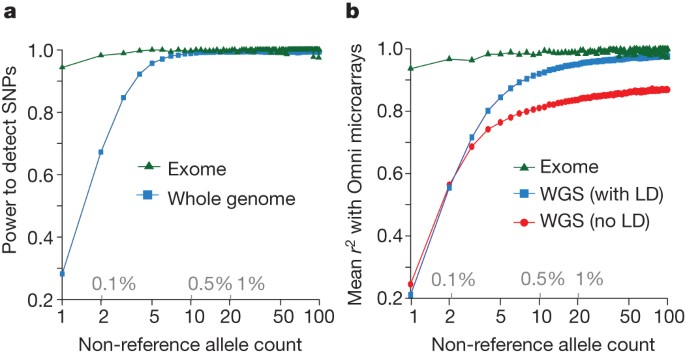
By comparison to external SNP and high-depth sequencing data, we estimate the power to detect SNPs present at a frequency of 1% in the study samples is 99.3% across the genome and 99.8% in the consensus exome target (Fig. 1a). Moreover, the power to detect SNPs at 0.1% frequency in the study is more than 90% in the exome and nearly 70% across the genome. The accuracy of individual genotype calls at heterozygous sites is more than 99% for common SNPs and 95% for SNPs at a frequency of 0.5% (Fig. 1b). By integrating linkage disequilibrium information, genotypes from low-coverage data are as accurate as those from high-depth exome data for SNPs with frequencies >1%. For very rare SNPs (≤0.1%, therefore present in one or two copies), there is no gain in genotype accuracy from incorporating linkage disequilibrium information and accuracy is lower. Variation among samples in genotype accuracy is primarily driven by sequencing depth (Supplementary Fig. 3) and technical issues such as sequencing platform and version (detectable by principal component analysis; Supplementary Fig. 4), rather than by population-level characteristics. The accuracy of inferred haplotypes at common SNPs was estimated by comparison to SNP data collected on mother–father–offspring trios for a subset of the samples. This indicates that a phasing (switch) error is made, on average, every 300–400 kilobases (kb) (Supplementary Fig. 5).
a, Power to detect SNPs as a function of variant count (and proportion) across the entire set of samples, estimated by comparison to independent SNP array data in the exome (green) and whole genome (blue). b, Genotype accuracy compared with the same SNP array data as a function of variant frequency, summarized by the r2 between true and inferred genotype (coded as 0, 1 and 2) within the exome (green), whole genome after haplotype integration (blue), and whole genome without haplotype integration (red). LD, linkage disequilibrium; WGS, whole-genome sequencing.
A key goal of the 1000 Genomes Project was to identify more than 95% of SNPs at 1% frequency in a broad set of populations. Our current resource includes ∼50%, 98% and 99.7% of the SNPs with frequencies of ∼0.1%, 1.0% and 5.0%, respectively, in ∼2,500 UK-sampled genomes (the Wellcome Trust-funded UK10K project), thus meeting this goal. However, coverage may be lower for populations not closely related to those studied. For example, our resource includes only 23.7%, 76.9% and 99.3% of the SNPs with frequencies of ∼0.1%, 1.0% and 5.0%, respectively, in ∼2,000 genomes sequenced in a study of the isolated population of Sardinia (the SardiNIA study).
Genetic variation within and between populations
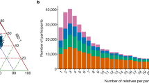
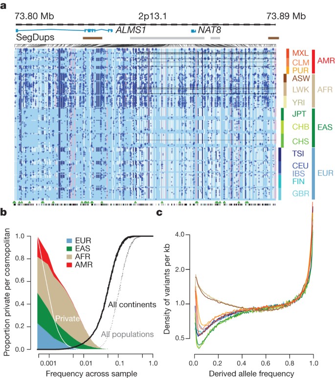
The integrated data set provides a detailed view of variation across several populations (illustrated in Fig. 2a). Most common variants (94% of variants with frequency ≥5% in Fig. 2a) were known before the current phase of the project and had their haplotype structure mapped through earlier projects2,9. By contrast, only 62% of variants in the range 0.5–5% and 13% of variants with frequencies of ≤0.5% had been described previously. For analysis, populations are grouped by the predominant component of ancestry: Europe (CEU (see Fig. 2a for definitions of this and other populations), TSI, GBR, FIN and IBS), Africa (YRI, LWK and ASW), East Asia (CHB, JPT and CHS) and the Americas (MXL, CLM and PUR). Variants present at 10% and above across the entire sample are almost all found in all of the populations studied. By contrast, 17% of low-frequency variants in the range 0.5–5% were observed in a single ancestry group, and 53% of rare variants at 0.5% were observed in a single population (Fig. 2b). Within ancestry groups, common variants are weakly differentiated (most within-group estimates of Wright’s fixation index (FST) are <1%; Supplementary Table 11), although below 0.5% frequency variants are up to twice as likely to be found within the same population compared with random samples from the ancestry group (Supplementary Fig. 6a). The degree of rare-variant differentiation varies between populations. For example, within Europe, the IBS and FIN populations carry excesses of rare variants (Supplementary Fig. 6b), which can arise through events such as recent bottlenecks10, ‘clan’ breeding structures11 and admixture with diverged populations12.
a, Summary of inferred haplotypes across a 100-kb region of chromosome 2 spanning the genes ALMS1 and NAT8, variation in which has been associated with kidney disease45. Each row represents an estimated haplotype, with the population of origin indicated on the right. Reference alleles are indicated by the light blue background. Variants (non-reference alleles) above 0.5% frequency are indicated by pink (typed on the high-density SNP array), white (previously known) and dark blue (not previously known). Low frequency variants (<0.5%) are indicated by blue crosses. Indels are indicated by green triangles and novel variants by dashes below. A large, low-frequency deletion (black line) spanning NAT8 is present in some populations. Multiple structural haplotypes mediated by segmental duplications are present at this locus, including copy number gains, which were not genotyped for this study. Within each population, haplotypes are ordered by total variant count across the region. Population abbreviations: ASW, people with African ancestry in Southwest United States; CEU, Utah residents with ancestry from Northern and Western Europe; CHB, Han Chinese in Beijing, China; CHS, Han Chinese South, China; CLM, Colombians in Medellin, Colombia; FIN, Finnish in Finland; GBR, British from England and Scotland, UK; IBS, Iberian populations in Spain; LWK, Luhya in Webuye, Kenya; JPT, Japanese in Tokyo, Japan; MXL, people with Mexican ancestry in Los Angeles, California; PUR, Puerto Ricans in Puerto Rico; TSI, Toscani in Italia; YRI, Yoruba in Ibadan, Nigeria. Ancestry-based groups: AFR, African; AMR, Americas; EAS, East Asian; EUR, European. b, The fraction of variants identified across the project that are found in only one population (white line), are restricted to a single ancestry-based group (defined as in a, solid colour), are found in all groups (solid black line) and all populations (dotted black line). c, The density of the expected number of variants per kilobase carried by a genome drawn from each population, as a function of variant frequency (see Supplementary Information). Colours as in a. Under a model of constant population size, the expected density is constant across the frequency spectrum.
Some common variants show strong differentiation between populations within ancestry-based groups (Supplementary Table 12), many of which are likely to have been driven by local adaptation either directly or through hitchhiking. For example, the strongest differentiation between African populations is within an NRSF (neuron-restrictive silencer factor) transcription-factor peak (PANC1 cell line)13, upstream of ST8SIA1 (difference in derived allele frequency LWK − YRI of 0.475 at rs7960970), whose product is involved in ganglioside generation14. Overall, we find a range of 17–343 SNPs (fewest = CEU − GBR, most = FIN − TSI) showing a difference in frequency of at least 0.25 between pairs of populations within an ancestry group.
The derived allele frequency distribution shows substantial divergence between populations below a frequency of 40% (Fig. 2c), such that individuals from populations with substantial African ancestry (YRI, LWK and ASW) carry up to three times as many low-frequency variants (0.5–5% frequency) as those of European or East Asian origin, reflecting ancestral bottlenecks in non-African populations15. However, individuals from all populations show an enrichment of rare variants (<0.5% frequency), reflecting recent explosive increases in population size and the effects of geographic differentiation6,16. Compared with the expectations from a model of constant population size, individuals from all populations show a substantial excess of high-frequency-derived variants (>80% frequency).
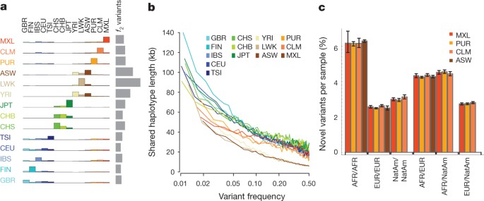
Because rare variants are typically recent, their patterns of sharing can reveal aspects of population history. Variants present twice across the entire sample (referred to as f2 variants), typically the most recent of informative mutations, are found within the same population in 53% of cases (Fig. 3a). However, between-population sharing identifies recent historical connections. For example, if one of the individuals carrying an f2 variant is from the Spanish population (IBS) and the other is not (referred to as IBS−X), the other individual is more likely to come from the Americas populations (48%, correcting for sample size) than from elsewhere in Europe (41%). Within the East Asian populations, CHS and CHB show stronger f2 sharing to each other (58% and 53% of CHS−X and CHB−X variants, respectively) than either does to JPT, but JPT is closer to CHB than to CHS (44% versus 35% of JPT−X variants). Within African-ancestry populations, the ASW are closer to the YRI (42% of ASW−X f2 variants) than the LWK (28%), in line with historical information17 and genetic evidence based on common SNPs18. Some sharing patterns are surprising; for example, 2.5% of the f2 FIN−X variants are shared with YRI or LWK populations.
a, Sharing of f2 variants, those found exactly twice across the entire sample, within and between populations. Each row represents the distribution across populations for the origin of samples sharing an f2 variant with the target population (indicated by the left-hand side). The grey bars represent the average number of f2 variants carried by a randomly chosen genome in each population. b, Median length of haplotype identity (excluding cryptically related samples and singleton variants, and allowing for up to two genotype errors) between two chromosomes that share variants of a given frequency in each population. Estimates are from 200 randomly sampled regions of 1 Mb each and up to 15 pairs of individuals for each variant. c, The average proportion of variants that are new (compared with the pilot phase of the project) among those found in regions inferred to have different ancestries within ASW, PUR, CLM and MXL populations. Error bars represent 95% bootstrap confidence intervals. NatAm, Native American.
Independent evidence about variant age comes from the length of the shared haplotypes on which they are found. We find, as expected, a negative correlation between variant frequency and the median length of shared haplotypes, such that chromosomes carrying variants at 1% frequency share haplotypes of 100–150 kb (typically 0.08–0.13 cM; Fig. 3b and Supplementary Fig. 7a), although the distribution is highly skewed and 2–5% of haplotypes around the rarest SNPs extend over 1 megabase (Mb) (Supplementary Fig. 7b, c). Haplotype phasing and genotype calling errors will limit the ability to detect long shared haplotypes, and the observed lengths are a factor of 2–3 times shorter than predicted by models that allow for recent explosive growth6 (Supplementary Fig. 7a). Nevertheless, the haplotype length for variants shared within and between populations is informative about relative allele age. Within populations and between populations in which there is recent shared ancestry (for example, through admixture and within continents), f2 variants typically lie on long shared haplotypes (median within ancestry group 103 kb; Supplementary Fig. 8). By contrast, between populations with no recent shared ancestry, f2 variants are present on very short haplotypes, for example, an average of 11 kb for FIN − YRI f2 variants (median between ancestry groups excluding admixture is 15 kb), and are therefore likely to reflect recurrent mutations and chance ancient coalescent events.
To analyse populations with substantial historical admixture, statistical methods were applied to each individual to infer regions of the genome with different ancestries. Populations and individuals vary substantially in admixture proportions. For example, the MXL population contains the greatest proportion of Native American ancestry (47% on average compared with 24% in CLM and 13% in PUR), but the proportion varies from 3% to 92% between individuals (Supplementary Fig. 9a). Rates of variant discovery, the ratio of non-synonymous to synonymous variation and the proportion of variants that are new vary systematically between regions with different ancestries. Regions of Native American ancestry show less variation, but a higher fraction of the variants discovered are novel (3.0% of variants per sample; Fig. 3c) compared with regions of European ancestry (2.6%). Regions of African ancestry show the highest rates of novelty (6.2%) and heterozygosity (Supplementary Fig. 9b, c).
The functional spectrum of human variation
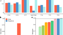
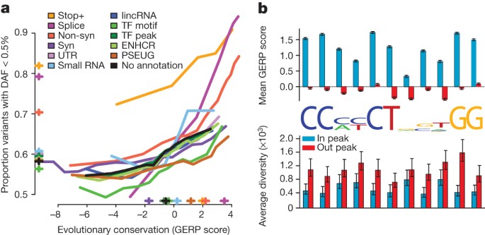
The phase I data enable us to compare, for different genomic features and variant types, the effects of purifying selection on evolutionary conservation19, the allele frequency distribution and the level of differentiation between populations. At the most highly conserved coding sites, 85% of non-synonymous variants and more than 90% of stop-gain and splice-disrupting variants are below 0.5% in frequency, compared with 65% of synonymous variants (Fig. 4a). In general, the rare variant excess tracks the level of evolutionary conservation for variants of most functional consequence, but varies systematically between types (for example, for a given level of conservation enhancer variants have a higher rare variant excess than variants in transcription-factor motifs). However, stop-gain variants and, to a lesser extent, splice-site disrupting changes, show increased rare-variant excess whatever the conservation of the base in which they occur, as such mutations can be highly deleterious whatever the level of sequence conservation. Interestingly, the least conserved splice-disrupting variants show similar rare-variant loads to synonymous and non-coding regions, suggesting that these alternative transcripts are under very weak selective constraint. Sites at which variants are observed are typically less conserved than average (for example, sites with non-synonymous variants are, on average, as conserved as third codon positions; Supplementary Fig. 10).
a, The relationship between evolutionary conservation (measured by GERP score19) and rare variant proportion (fraction of all variants with derived allele frequency (DAF) < 0.5%) for variants occurring in different functional elements and with different coding consequences. Crosses indicate the average GERP score at variant sites (x axis) and the proportion of rare variants (y axis) in each category. ENHCR, enhancer; lincRNA, large intergenic non-coding RNA; non-syn, non-synonymous; PSEUG, pseudogene; syn, synonymous; TF, transcription factor. b, Levels of evolutionary conservation (mean GERP score, top) and genetic diversity (per-nucleotide pairwise differences, bottom) for sequences matching the CTCF-binding motif within CTCF-binding peaks, as identified experimentally by ChIP-seq in the ENCODE project13 (blue) and in a matched set of motifs outside peaks (red). The logo plot shows the distribution of identified motifs within peaks. Error bars represent ±2 s.e.m.
A simple way of estimating the segregating load arising from rare, deleterious mutations across a set of genes comes from comparing the ratios of non-synonymous to synonymous variants in different frequency ranges. The non-synonymous to synonymous ratio among rare (<0.5%) variants is typically in the range 1–2, and among common variants in the range 0.5–1.5, suggesting that 25–50% of rare non-synonymous variants are deleterious. However, the segregating rare load among gene groups in KEGG pathways20 varies substantially (Supplementary Fig. 11a and Supplementary Table 13). Certain groups (for example, those involving extracellular matrix (ECM)–receptor interactions, DNA replication and the pentose phosphate pathway) show a substantial excess of rare coding mutations, which is only weakly correlated with the average degree of evolutionary conservation. Pathways and processes showing an excess of rare functional variants vary between continents (Supplementary Fig. 11b). Moreover, the excess of rare non-synonymous variants is typically higher in populations of European and East Asian ancestry (for example, the ECM–receptor interaction pathway load is strongest in European populations). Other groups of genes (such as those associated with allograft rejection) have a high non-synonymous to synonymous ratio in common variants, potentially indicating the effects of positive selection.
Genome-wide data provide important insights into the rates of functional polymorphism in the non-coding genome. For example, we consider motifs matching the consensus for the transcriptional repressor CTCF, which has a well-characterized and highly conserved binding motif21. Within CTCF-binding peaks experimentally defined by chromatin-immunoprecipitation sequencing (ChIP-seq), the average levels of conservation within the motif are comparable to third codon positions, whereas there is no conservation outside peaks (Fig. 4b). Within peaks, levels of genetic diversity are typically reduced 25–75%, depending on the position in the motif (Fig. 4b). Unexpectedly, the reduction in diversity at some degenerate positions, for example, at position 8 in the motif, is as great as that at non-degenerate positions, suggesting that motif degeneracy may not have a simple relationship with functional importance. Variants within peaks show a weak but consistent excess of rare variation (proportion with frequency <0.5% is 61% within peaks compared with 58% outside peaks; Supplementary Fig. 12), supporting the hypothesis that regulatory sequences contain substantial amounts of weakly deleterious variation.
Purifying selection can also affect population differentiation if its strength and efficacy vary among populations. Although the magnitude of the effect is weak, non-synonymous variants consistently show greater levels of population differentiation than synonymous variants, for variants of frequencies of less than 10% (Supplementary Fig. 13).
Uses of 1000 Genomes Project data in medical genetics
Data from the 1000 Genomes Project are widely used to screen variants discovered in exome data from individuals with genetic disorders22 and in cancer genome projects23. The enhanced catalogue presented here improves the power of such screening. Moreover, it provides a ‘null expectation’ for the number of rare, low-frequency and common variants with different functional consequences typically found in randomly sampled individuals from different populations.
Estimates of the overall numbers of variants with different sequence consequences are comparable to previous values1,20,21,22 (Supplementary Table 14). However, only a fraction of these are likely to be functionally relevant. A more accurate picture of the number of functional variants is given by the number of variants segregating at conserved positions (here defined as sites with a genomic evolutionary rate profiling (GERP)19 conservation score of >2), or where the function (for example, stop-gain variants) is strong and independent of conservation (Table 2). We find that individuals typically carry more than 2,500 non-synonymous variants at conserved positions, 20–40 variants identified as damaging24 at conserved sites and about 150 loss-of-function (LOF) variants (stop-gains, frameshift indels in coding sequence and disruptions to essential splice sites). However, most of these are common (>5%) or low-frequency (0.5–5%), such that the numbers of rare (<0.5%) variants in these categories (which might be considered as pathological candidates) are much lower; 130–400 non-synonymous variants per individual, 10–20 LOF variants, 2–5 damaging mutations, and 1–2 variants identified previously from cancer genome sequencing25. By comparison with synonymous variants, we can estimate the excess of rare variants; those mutations that are sufficiently deleterious that they will never reach high frequency. We estimate that individuals carry an excess of 76–190 rare deleterious non-synonymous variants and up to 20 LOF and disease-associated variants. Interestingly, the overall excess of low-frequency variants is similar to that of rare variants (Table 2). Because many variants contributing to disease risk are likely to be segregating at low frequency, we recommend that variant frequency be considered when using the resource to identify pathological candidates.
The combination of variation data with information about regulatory function13 can potentially improve the power to detect pathological non-coding variants. We find that individuals typically contain several thousand variants (and several hundred rare variants) in conserved (GERP conservation score >2) untranslated regions (UTR), non-coding RNAs and transcription-factor-binding motifs (Table 2). Within experimentally defined transcription-factor-binding sites, individuals carry 700–900 conserved motif losses (for the transcription factors analysed, see Supplementary Information), of which 18–69 are rare (<0.5%) and show strong evidence for being selected against. Motif gains are rarer (∼200 per individual at conserved sites), but they also show evidence for an excess of rare variants compared with conserved sites with no functional annotation (Table 2). Many of these changes are likely to have weak, slightly deleterious effects on gene regulation and function.
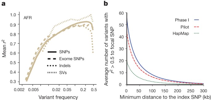
A second major use of the 1000 Genomes Project data in medical genetics is imputing genotypes in existing genome-wide association studies (GWAS)26. For common variants, the accuracy of using the phase I data to impute genotypes at sites not on the original GWAS SNP array is typically 90–95% in non-African and approximately 90% in African-ancestry genomes (Fig. 5a and Supplementary Fig. 14a), which is comparable to the accuracy achieved with high-quality benchmark haplotypes (Supplementary Fig. 14b). Imputation accuracy is similar for intergenic SNPs, exome SNPs, indels and large deletions (Supplementary Fig. 14c), despite the different amounts of information about such variants and accuracy of genotypes. For low-frequency variants (1–5%), imputed genotypes have between 60% and 90% accuracy in all populations, including those with admixed ancestry (also comparable to the accuracy from trio-phased haplotypes; Supplementary Fig. 14b).
a, Accuracy of imputation of genome-wide SNPs, exome SNPs and indels (using sites on the Illumina 1 M array) into ten individuals of African ancestry (three LWK, four Masaai from Kinyawa, Kenya (MKK), two YRI), sequenced to high coverage by an independent technology3. Only indels in regions of high sequence complexity with frequency >1% are analysed. Deletion imputation accuracy estimated by comparison to array data46 (note that this is for a different set of individuals, although with a similar ancestry, but included on the same plot for clarity). Accuracy measured by squared Pearson correlation coefficient between imputed and true dosage across all sites in a frequency range estimated from the 1000 Genomes data. Lines represent whole-genome SNPs (solid), exome SNPs (long dashes), short indels (dotted) and large deletions (short dashes). SV, structural variants. b, The average number of variants in linkage disequilibrium (r2 > 0.5 among EUR) to focal SNPs identified in GWAS47 as a function of distance from the index SNP. Lines indicate the number of HapMap (green), pilot (red) and phase I (blue) variants.
Imputation has two primary uses: fine-mapping existing association signals and detecting new associations. GWAS have had only a few examples of successful fine-mapping to single causal variants27,28, often because of extensive haplotype structure within regions of association29,30. We find that, in Europeans, each previously reported GWAS signal31 is, on average, in linkage disequilibrium (r2 ≥ 0.5) with 56 variants: 51.5 SNPs and 4.5 indels. In 19% of cases at least one of these variants changes the coding sequence of a nearby gene (compared with 12% in control variants matched for frequency, distance to nearest gene and ascertainment in GWAS arrays) and in 65% of cases at least one of these is at a site with GERP >2 (68% in matched controls). The size of the associated region is typically <200 kb in length (Fig. 5b). Our observations suggest that trans-ethnic fine-mapping experiments are likely to be especially valuable: among the 56 variants that are in strong linkage disequilibrium with a typical GWAS signal, approximately 15 show strong disequilibrium across our four continental groupings (Supplementary Table 15). Our current resource increases the number of variants in linkage disequilibrium with each GWAS signal by 25% compared with the pilot phase of the project and by greater than twofold compared with the HapMap resource.
Discussion
The success of exome sequencing in Mendelian disease genetics32 and the discovery of rare and low-frequency disease-associated variants in genes associated with complex diseases27,33,34 strongly support the hypothesis that, in addition to factors such as epistasis35,36 and gene–environment interactions37, many other genetic risk factors of substantial effect size remain to be discovered through studies of rare variation. The data generated by the 1000 Genomes Project not only aid the interpretation of all genetic-association studies, but also provide lessons on how best to design and analyse sequencing-based studies of disease.
The use and cost-effectiveness of collecting several data types (low-coverage whole-genome sequence, targeted exome data, SNP genotype data) for finding variants and reconstructing haplotypes are demonstrated here. Exome capture provides private and rare variants that are missed by low-coverage data (approximately 60% of the singleton variants in the sample were detected only from exome data compared with 5% detected only from low-coverage data; Supplementary Fig. 15). However, whole-genome data enable characterization of functional non-coding variation and accurate haplotype estimation, which are essential for the analysis of cis-effects around genes, such as those arising from variation in upstream regulatory regions38. There are also benefits from integrating SNP array data, for example, to improve genotype estimation39 and to aid haplotype estimation where array data have been collected on additional family members. In principle, any sources of genotype information (for example, from array CGH) could be integrated using the statistical methods developed here.
Major methodological advances in phase I, including improved methods for detecting and genotyping variants40, statistical and machine-learning methods for evaluating the quality of candidate variant calls, modelling of genotype likelihoods and performing statistical haplotype integration41, have generated a high-quality resource. However, regions of low sequence complexity, satellite regions, large repeats and many large-scale structural variants, including copy-number polymorphisms, segmental duplications and inversions (which constitute most of the ‘inaccessible genome’), continue to present a major challenge for short-read technologies. Some issues are likely to be improved by methodological developments such as better modelling of read-level errors, integrating de novo assembly42,43 and combining multiple sources of information to aid genotyping of structurally diverse regions40,44. Importantly, even subtle differences in data type, data processing or algorithms may lead to systematic differences in false-positive and false-negative error modes between samples. Such differences complicate efforts to compare genotypes between sequencing studies. Moreover, analyses that naively combine variant calls and genotypes across heterogeneous data sets are vulnerable to artefact. Analyses across multiple data sets must therefore either process them in standard ways or use meta-analysis approaches that combine association statistics (but not raw data) across studies.
Finally, the analysis of low-frequency variation demonstrates both the pervasive effects of purifying selection at functionally relevant sites in the genome and how this can interact with population history to lead to substantial local differentiation, even when standard metrics of structure such as FST are very small. The effect arises primarily because rare variants tend to be recent and thus geographically restricted6,7,8. The implication is that the interpretation of rare variants in individuals with a particular disease should be within the context of the local (either geographic or ancestry-based) genetic background. Moreover, it argues for the value of continuing to sequence individuals from diverse populations to characterize the spectrum of human genetic variation and support disease studies across diverse groups. A further 1,500 individuals from 12 new populations, including at least 15 high-depth trios, will form the final phase of this project.
Methods Summary
All details concerning sample collection, data generation, processing and analysis can be found in the Supplementary Information. Supplementary Fig. 1 summarizes the process and indicates where relevant details can be found.
References
Tennessen, J. A. et al. Evolution and functional impact of rare coding variation from deep sequencing of human exomes. Science 337, 64–69 (2012)
The 1000 Genomes Project Consortium. A map of human genome variation from population-scale sequencing. Nature 467, 1061–1073 (2010)
Drmanac, R. et al. Human genome sequencing using unchained base reads on self-assembling DNA nanoarrays. Science 327, 78–81 (2010)
Mills, R. E. et al. Mapping copy number variation by population-scale genome sequencing. Nature 470, 59–65 (2011)
Marth, G. T. et al. The functional spectrum of low-frequency coding variation. Genome Biol. 12, R84 (2011)
Nelson, M. R. et al. An abundance of rare functional variants in 202 drug target genes sequenced in 14,002 people. Science 337, 100–104 (2012)
Mathieson, I. & McVean, G. Differential confounding of rare and common variants in spatially structured populations. Nature Genet. 44, 243–246 (2012)
Gravel, S. et al. Demographic history and rare allele sharing among human populations. Proc. Natl Acad. Sci. USA 108, 11983–11988 (2011)
The International HapMap Consortium. A second generation human haplotype map of over 3.1 million SNPs. Nature 449, 851–861 (2007)
Salmela, E. et al. Genome-wide analysis of single nucleotide polymorphisms uncovers population structure in Northern Europe. PLoS ONE 3, e3519 (2008)
Lupski, J. R., Belmont, J. W., Boerwinkle, E. & Gibbs, R. A. Clan genomics and the complex architecture of human disease. Cell 147, 32–43 (2011)
Lawson, D. J., Hellenthal, G., Myers, S. & Falush, D. Inference of population structure using dense haplotype data. PLoS Genet. 8, e1002453 (2012)
ENCODE Project Consortium. A user’s guide to the encyclopedia of DNA elements (ENCODE). PLoS Biol. 9, e1001046 (2011)
Sasaki, K. et al. Expression cloning of a novel Galβ(1–3/1–4)GlcNAc α2,3-sialyltransferase using lectin resistance selection. J. Biol. Chem. 268, 22782–22787 (1993)
Marth, G. et al. Sequence variations in the public human genome data reflect a bottlenecked population history. Proc. Natl Acad. Sci. USA 100, 376–381 (2003)
Keinan, A. & Clark, A. G. Recent explosive human population growth has resulted in an excess of rare genetic variants. Science 336, 740–743 (2012)
Hall, G. M. Slavery and African Ethnicities in the Americas: Restoring the Links (Univ. North Carolina Press, 2005)
Bryc, K. et al. Genome-wide patterns of population structure and admixture in West Africans and African Americans. Proc. Natl Acad. Sci. USA 107, 786–791 (2010)
Davydov, E. V. et al. Identifying a high fraction of the human genome to be under selective constraint using GERP++. PLOS Comput. Biol. 6, e1001025 (2010)
Kanehisa, M., Goto, S., Sato, Y., Furumichi, M. & Tanabe, M. KEGG for integration and interpretation of large-scale molecular data sets. Nucleic Acids Res. 40, D109–D114 (2012)
Kim, T. H. et al. Analysis of the vertebrate insulator protein CTCF-binding sites in the human genome. Cell 128, 1231–1245 (2007)
Bamshad, M. J. et al. Exome sequencing as a tool for Mendelian disease gene discovery. Nature Rev. Genet. 12, 745–755 (2011)
Cancer Genome Altas Research Network. Integrated genomic analyses of ovarian carcinoma. Nature 474, 609–615 (2011)
Stenson, P. D. et al. The Human Gene Mutation Database: 2008 update. Genome Med. 1, 13 (2009)
Forbes, S. A. et al. COSMIC: mining complete cancer genomes in the Catalogue of Somatic Mutations in Cancer. Nucleic Acids Res. 39, D945–D950 (2011)
Howie, B., Marchini, J. & Stephens, M. Genotype imputation with thousands of genomes. G3 (Bethesda) 1, 457–470 (2011)
Sanna, S. et al. Fine mapping of five loci associated with low-density lipoprotein cholesterol detects variants that double the explained heritability. PLoS Genet. 7, e1002198 (2011)
Gregory, A. P., Dendrou, C. A., Bell, J., McVean, G. & Fugger, L. TNF receptor 1 genetic risk mirrors outcome of anti-TNF therapy in multiple sclerosis. Nature 488, 508–511 (2012)
Hassanein, M. T. et al. Fine mapping of the association with obesity at the FTO locus in African-derived populations. Hum. Mol. Genet. 19, 2907–2916 (2010)
Maller, J. The Wellcome Trust Case Control Consortium. Fine mapping of 14 loci identified through genome-wide association analyses. Nature Genet. (in the press)
Hindorff, L. A. et al. Potential etiologic and functional implications of genome-wide association loci for human diseases and traits. Proc. Natl Acad. Sci. USA 106, 9362–9367 (2009)
Bamshad, M. J. et al. The Centers for Mendelian Genomics: A new large-scale initiative to identify the genes underlying rare Mendelian conditions. Am. J. Med. Genet. A. (2012)
Momozawa, Y. et al. Resequencing of positional candidates identifies low frequency IL23R coding variants protecting against inflammatory bowel disease. Nature Genet. 43, 43–47 (2011)
Raychaudhuri, S. et al. A rare penetrant mutation in CFH confers high risk of age-related macular degeneration. Nature Genet. 43, 1232–1236 (2011)
Strange, A. et al. A genome-wide association study identifies new psoriasis susceptibility loci and an interaction between HLA-C and ERAP1. Nature Genet. 42, 985–990 (2010)
Zuk, O., Hechter, E., Sunyaev, S. R. & Lander, E. S. The mystery of missing heritability: Genetic interactions create phantom heritability. Proc. Natl Acad. Sci. USA 109, 1193–1198 (2012)
Thomas, D. Gene-environment-wide association studies: emerging approaches. Nature Rev. Genet. 11, 259–272 (2010)
Degner, J. F. et al. DNase I sensitivity QTLs are a major determinant of human expression variation. Nature 482, 390–394 (2012)
Flannick, J. et al. Efficiency and power as a function of sequence coverage, SNP array density, and imputation. PLOS Comput. Biol. 8, e1002604 (2012)
Handsaker, R. E., Korn, J. M., Nemesh, J. & McCarroll, S. A. Discovery and genotyping of genome structural polymorphism by sequencing on a population scale. Nature Genet. 43, 269–276 (2011)
Li, Y., Sidore, C., Kang, H. M., Boehnke, M. & Abecasis, G. R. Low-coverage sequencing: implications for design of complex trait association studies. Genome Res. 21, 940–951 (2011)
Iqbal, Z., Caccamo, M., Turner, I., Flicek, P. & McVean, G. De novo assembly and genotyping of variants using colored de Bruijn graphs. Nature Genet. 44, 226–232 (2012)
Simpson, J. T. & Durbin, R. Efficient construction of an assembly string graph using the FM-index. Bioinformatics 26, i367–i373 (2010)
Sudmant, P. H. et al. Diversity of human copy number variation and multicopy genes. Science 330, 641–646 (2010)
Chambers, J. C. et al. Genetic loci influencing kidney function and chronic kidney disease. Nature Genet. 42, 373–375 (2010)
Conrad, D. F. et al. Origins and functional impact of copy number variation in the human genome. Nature 464, 704–712 (2010)
Hindorff, L. A. et al. A Catalog of Published Genome-Wide Association Studies. Available at http://www.genome.gov/gwastudies (accessed, September 2012)
Acknowledgements
We thank many people who contributed to this project: A. Naranjo, M. V. Parra and C. Duque for help with the collection of the Colombian samples; N. Kälin and F. Laplace for discussions; A. Schlattl and T. Zichner for assistance in managing data sets; E. Appelbaum, H. Arbery, E. Birney, S. Bumpstead, J. Camarata, J. Carey, G. Cochrane, M. DaSilva, S. Dökel, E. Drury, C. Duque, K. Gyaltsen, P. Jokinen, B. Lenz, S. Lewis, D. Lu, A. Naranjo, S. Ott, I. Padioleau, M. V. Parra, N. Patterson, A. Price, L. Sadzewicz, S. Schrinner, N. Sengamalay, J. Sullivan, F. Ta, Y. Vaydylevich, O. Venn, K. Watkins and A. Yurovsky for assistance, discussion and advice. We thank the people who generously contributed their samples, from these populations: Yoruba in Ibadan, Nigeria; the Han Chinese in Beijing, China; the Japanese in Tokyo, Japan; the Utah CEPH community; the Luhya in Webuye, Kenya; people with African ancestry in the Southwest United States; the Toscani in Italia; people with Mexican ancestry in Los Angeles, California; the Southern Han Chinese in China; the British in England and Scotland; the Finnish in Finland; the Iberian Populations in Spain; the Colombians in Medellin, Colombia; and the Puerto Ricans in Puerto Rico. This research was supported in part by Wellcome Trust grants WT098051 to R.M.D., M.E.H. and C.T.S.; WT090532/Z/09/Z, WT085475/Z/08/Z and WT095552/Z/11/Z to P.Do.; WT086084/Z/08/Z and WT090532/Z/09/Z to G.A.M.; WT089250/Z/09/Z to I.M.; WT085532AIA to P.F.; Medical Research Council grant G0900747(91070) to G.A.M.; British Heart Foundation grant RG/09/12/28096 to C.A.A.; the National Basic Research Program of China (973 program no. 2011CB809201, 2011CB809202 and 2011CB809203); the Chinese 863 program (2012AA02A201); the National Natural Science Foundation of China (30890032, 31161130357); the Shenzhen Key Laboratory of Transomics Biotechnologies (CXB201108250096A); the Shenzhen Municipal Government of China (grants ZYC200903240080A and ZYC201105170397A); Guangdong Innovative Research Team Program (no. 2009010016); BMBF grant 01GS08201 to H.Le.; BMBF grant 0315428A to R.H.; the Max Planck Society; Swiss National Science Foundation 31003A_130342 to E.T.D.; Swiss National Science Foundation NCCR ‘Frontiers in Genetics’ grant to E.T.D.; Louis Jeantet Foundation grant to E.T.D.; Biotechnology and Biological Sciences Research Council (BBSRC) grant BB/I021213/1 to A.R.-L.; German Research Foundation (Emmy Noether Fellowship KO 4037/1-1) to J.O.K.; Netherlands Organization for Scientific Research VENI grant 639.021.125 to K.Y.; Beatriu de Pinos Program grants 2006BP-A 10144 and 2009BP-B 00274 to M.V.; Israeli Science Foundation grant 04514831 to E.H.; Genome Québec and the Ministry of Economic Development, Innovation and Trade grant PSR-SIIRI-195 to P.Aw.; National Institutes of Health (NIH) grants UO1HG5214, RC2HG5581 and RO1MH84698 to G.R.A.; R01HG4719 and R01HG3698 to G.T.M; RC2HG5552 and UO1HG6513 to G.R.A. and G.T.M.; R01HG4960 and R01HG5701 to B.L.B.; U01HG5715 to C.D.B. and A.G.C.; T32GM8283 to D.Cl.; U01HG5208 to M.J.D.; U01HG6569 to M.A.D.; R01HG2898 and R01CA166661 to S.E.D.; UO1HG5209, UO1HG5725 and P41HG4221 to C.Le.; P01HG4120 to E.E.E.; U01HG5728 to Yu.F.; U54HG3273 and U01HG5211 to R.A.G.; R01HL95045 to S.B.G.; U41HG4568 to S.J.K.; P41HG2371 to W.J.K.; ES015794, AI077439, HL088133 and HL078885 to E.G.B.; RC2HL102925 to S.B.G. and D.M.A.; R01GM59290 to L.B.J. and M.A.B.; U54HG3067 to E.S.L. and S.B.G.; T15LM7033 to B.K.M.; T32HL94284 to J.L.R.-F.; DP2OD6514 and BAA-NIAID-DAIT-NIHAI2009061 to P.C.S.; T32GM7748 to X.S.; U54HG3079 to R.K.W.; UL1RR024131 to R.D.H.; HHSN268201100040C to the Coriell Institute for Medical Research; a Sandler Foundation award and an American Asthma Foundation award to E.G.B.; an IBM Open Collaborative Research Program award to Y.B.; an A.G. Leventis Foundation scholarship to D.K.X.; a Wolfson Royal Society Merit Award to P.Do.; a Howard Hughes Medical Institute International Fellowship award to P.H.S.; a grant from T. and V. Stanley to S.C.Y.; and a Mary Beryl Patch Turnbull Scholar Program award to K.C.B. E.H. is a faculty fellow of the Edmond J. Safra Bioinformatics program at Tel-Aviv University. E.E.E. and D.H. are investigators of the Howard Hughes Medical Institute. M.V.G. is a long-term fellow of EMBO.
Author information
Authors and Affiliations
Consortia
Contributions
Details of author contributions can be found in the author list.
Corresponding author
Ethics declarations
Competing interests
The authors declare competing financial interests: P.Aw. is an adviser for Ancestry.com; E.T.D. is an adviser for DNAnexus; A.Cha. is on the scientific advisory board for Affymetrix; C.D.B. is on the scientific advisory boards for Personalis, Inc., Ancestry.com, Locus Development and the 23andMe.com project ‘Roots into the future’; D.H. is on the scientific advisory board for Pacific Biosciences; E.E.E. is on the scientific advisory boards for Pacific Biosciences, Inc., SynapDx Corp, and DNAnexus, Inc.; P.F. is on the scientific advisory board for Omicia, Inc.; C.Le. is on the scientific advisory board for BioNano Genomics and is a senior scientific adviser for Samsung; E.R.M. holds shares in Life Technologies and serves on Illumina’s Speaker’s Bureau; R.A.G. and D.M. hold a co-investment with Life Technologies; J.K.B., C.J.D., J.Go., J.P.S., T.W., B.Wo. and Y.Zha. work at Affymetrix; J.K.B. works at Ancestry.com; N.Ho. works at Life Technologies; F.M.D. used to work and hold shares at Life Technologies; W.J.K. works at Kent Informatics; B.Ba., M.Bau., D.R.B., R.K.C., T.C., M.E., S.H., S.K., L.M., J.P. and R.Sh. work at Illumina.
Additional information
All primary data, alignments, individual call sets, consensus call sets, integrated haplotypes with genotype likelihoods and supporting data including details of validation are available from the project website (http://www.1000genomes.org). Variant and haplotypes for specific genomic regions and specific samples can be viewed and downloaded through the project browser (http://browser.1000genomes.org/).Common project variants with no known medical impact have been compiled by dbSNP for filtering (http://www.ncbi.nlm.nih.gov/variation/docs/human_variation_vcf/).
(Participants are arranged by project role, then by institution alphabetically, and finally alphabetically within institutions except for Principal Investigators and Project Leaders, as indicated.)
Supplementary information
Supplementary Information
This fie contains Supplementary Text and Data 1-11, Supplementary References, Supplementary Tables 1-15 and Supplementary Figures 1-15 (see Contents for details). (PDF 4567 kb)
Rights and permissions
This article is distributed under the terms of the Creative Commons Attribution-Non-Commercial-Share Alike licence (http://creativecommons.org/licenses/by-nc-sa/3.0/), which permits distribution, and reproduction in any medium, provided the original author and source are credited. This licence does not permit commercial exploitation, and derivative works must be licensed under the same or similar licence.
About this article
Cite this article
The 1000 Genomes Project Consortium. An integrated map of genetic variation from 1,092 human genomes. Nature 491, 56–65 (2012). https://doi.org/10.1038/nature11632
Received:
Accepted:
Published:
Issue Date:
DOI: https://doi.org/10.1038/nature11632


