iBet uBet web content aggregator. Adding the entire web to your favor.


Link to original content: http://www.ncbi.nlm.nih.gov/pubmed/29934920
Convolutional neural networks: an overview and application in radiology - PubMed Skip to main page content
U.S. flag

An official website of the United States government

Dot gov

The .gov means it’s official.
Federal government websites often end in .gov or .mil. Before sharing sensitive information, make sure you’re on a federal government site.

Https

The site is secure.
The https:// ensures that you are connecting to the official website and that any information you provide is encrypted and transmitted securely.

Access keys NCBI Homepage MyNCBI Homepage Main Content Main Navigation
Review
. 2018 Aug;9(4):611-629.
doi: 10.1007/s13244-018-0639-9. Epub 2018 Jun 22.

Convolutional neural networks: an overview and application in radiology

Affiliations
Review

Convolutional neural networks: an overview and application in radiology

Rikiya Yamashita et al. Insights Imaging. 2018 Aug.

Abstract

Convolutional neural network (CNN), a class of artificial neural networks that has become dominant in various computer vision tasks, is attracting interest across a variety of domains, including radiology. CNN is designed to automatically and adaptively learn spatial hierarchies of features through backpropagation by using multiple building blocks, such as convolution layers, pooling layers, and fully connected layers. This review article offers a perspective on the basic concepts of CNN and its application to various radiological tasks, and discusses its challenges and future directions in the field of radiology. Two challenges in applying CNN to radiological tasks, small dataset and overfitting, will also be covered in this article, as well as techniques to minimize them. Being familiar with the concepts and advantages, as well as limitations, of CNN is essential to leverage its potential in diagnostic radiology, with the goal of augmenting the performance of radiologists and improving patient care. KEY POINTS: • Convolutional neural network is a class of deep learning methods which has become dominant in various computer vision tasks and is attracting interest across a variety of domains, including radiology. • Convolutional neural network is composed of multiple building blocks, such as convolution layers, pooling layers, and fully connected layers, and is designed to automatically and adaptively learn spatial hierarchies of features through a backpropagation algorithm. • Familiarity with the concepts and advantages, as well as limitations, of convolutional neural network is essential to leverage its potential to improve radiologist performance and, eventually, patient care.

Keywords: Convolutional neural network; Deep learning; Machine learning; Medical imaging; Radiology.


Figures

Fig. 1
Fig. 1
An overview of a convolutional neural network (CNN) architecture and the training process. A CNN is composed of a stacking of several building blocks: convolution layers, pooling layers (e.g., max pooling), and fully connected (FC) layers. A model’s performance under particular kernels and weights is calculated with a loss function through forward propagation on a training dataset, and learnable parameters, i.e., kernels and weights, are updated according to the loss value through backpropagation with gradient descent optimization algorithm. ReLU, rectified linear unit
Fig. 2
Fig. 2
A computer sees an image as an array of numbers. The matrix on the right contains numbers between 0 and 255, each of which corresponds to the pixel brightness in the left image. Both are overlaid in the middle image. The source image was downloaded via http://yann.lecun.com/exdb/mnist
Fig. 3
Fig. 3
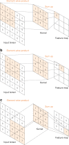
ac An example of convolution operation with a kernel size of 3 × 3, no padding, and a stride of 1. A kernel is applied across the input tensor, and an element-wise product between each element of the kernel and the input tensor is calculated at each location and summed to obtain the output value in the corresponding position of the output tensor, called a feature map. d Examples of how kernels in convolution layers extract features from an input tensor are shown. Multiple kernels work as different feature extractors, such as a horizontal edge detector (top), a vertical edge detector (middle), and an outline detector (bottom). Note that the left image is an input, those in the middle are kernels, and those in the right are output feature maps
Fig. 3
Fig. 3
ac An example of convolution operation with a kernel size of 3 × 3, no padding, and a stride of 1. A kernel is applied across the input tensor, and an element-wise product between each element of the kernel and the input tensor is calculated at each location and summed to obtain the output value in the corresponding position of the output tensor, called a feature map. d Examples of how kernels in convolution layers extract features from an input tensor are shown. Multiple kernels work as different feature extractors, such as a horizontal edge detector (top), a vertical edge detector (middle), and an outline detector (bottom). Note that the left image is an input, those in the middle are kernels, and those in the right are output feature maps
Fig. 4
Fig. 4
A convolution operation with zero padding so as to retain in-plane dimensions. Note that an input dimension of 5 × 5 is kept in the output feature map. In this example, a kernel size and a stride are set as 3 × 3 and 1, respectively
Fig. 5
Fig. 5
Activation functions commonly applied to neural networks: a rectified linear unit (ReLU), b sigmoid, and c hyperbolic tangent (tanh)
Fig. 6
Fig. 6
a An example of max pooling operation with a filter size of 2 × 2, no padding, and a stride of 2, which extracts 2 × 2 patches from the input tensors, outputs the maximum value in each patch, and discards all the other values, resulting in downsampling the in-plane dimension of an input tensor by a factor of 2. b Examples of the max pooling operation on the same images in Fig. 3b. Note that images in the upper row are downsampled by a factor of 2, from 26 × 26 to 13 × 13
Fig. 7
Fig. 7
Gradient descent is an optimization algorithm that iteratively updates the learnable parameters so as to minimize the loss, which measures the distance between an output prediction and a ground truth label. The gradient of the loss function provides the direction in which the function has the steepest rate of increase, and all parameters are updated in the negative direction of the gradient with a step size determined based on a learning rate
Fig. 8
Fig. 8
Available data are typically split into three sets: a training, a validation, and a test set. A training set is used to train a network, where loss values are calculated via forward propagation and learnable parameters are updated via backpropagation. A validation set is used to monitor the model performance during the training process, fine-tune hyperparameters, and perform model selection. A test set is ideally used only once at the very end of the project in order to evaluate the performance of the final model that is fine-tuned and selected on the training process with training and validation sets
Fig. 9
Fig. 9
A routine check for recognizing overfitting is to monitor the loss on the training and validation sets during the training iteration. If the model performs well on the training set compared to the validation set, then the model has been overfit to the training data. If the model performs poorly on both training and validation sets, then the model has been underfit to the data. Although the longer a network is trained, the better it performs on the training set, at some point, the network fits too well to the training data and loses its capability to generalize
Fig. 10
Fig. 10
Transfer learning is a common and effective strategy to train a network on a small dataset, where a network is pretrained on an extremely large dataset, such as ImageNet, then reused and applied to the given task of interest. A fixed feature extraction method is a process to remove FC layers from a pretrained network and while maintaining the remaining network, which consists of a series of convolution and pooling layers, referred to as the convolutional base, as a fixed feature extractor. In this scenario, any machine learning classifier, such as random forests and support vector machines, as well as the usual FC layers, can be added on top of the fixed feature extractor, resulting in training limited to the added classifier on a given dataset of interest. A fine-tuning method, which is more often applied to radiology research, is to not only replace FC layers of the pretrained model with a new set of FC layers to retrain them on a given dataset, but to fine-tune all or part of the kernels in the pretrained convolutional base by means of backpropagation. FC, fully connected
Fig. 11
Fig. 11
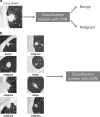
A schematic illustration of a classification system with CNN and representative examples of its training data. a Classification system with CNN in the deployment phase. b, c Training data used in training phase
Fig. 11
Fig. 11
A schematic illustration of a classification system with CNN and representative examples of its training data. a Classification system with CNN in the deployment phase. b, c Training data used in training phase
Fig. 12
Fig. 12
A schematic illustration of the system for segmenting a uterus with a malignant tumor and representative examples of its training data. a Segmentation system with CNN in deployment phase. b Training data used in the training phase. Note that original images and corresponding manual segmentations are arranged next to each other
Fig. 13
Fig. 13
A schematic illustration of the system for denoising an ultra-low-dose CT (ULDCT) image of phantom and representative examples of its training data. a Denoising system with CNN in deployment phase. b Training data used in training phase. SDCT, standard-dose CT
Fig. 14
Fig. 14
An example of a class activation map (CAM) [58]. A CNN network trained on ImageNet classified the left image as a “bridge pier”. A heatmap for the category of “bridge pier”, generated by a method called Grad-CAM [59], is superimposed (right image), which indicates the discriminative image regions used by the CNN for the classification
Fig. 15
Fig. 15
An adversarial example demonstrated by Goodfellow et al. [61]. A network classified the object in the left image as a “panda” with 57.7% confidence. By adding a very small amount of carefully constructed noise (middle image), the network misclassified the object as a “gibbon” with 99.3% confidence on the right image without a visible change to a human. Reprinted with permission from “Explaining and harnessing adversarial examples” by Goodfellow et al. [61]

Similar articles

Cited by

References

    1. LeCun Y, Bengio Y, Hinton G. Deep learning. Nature. 2015;521:436–444. doi: 10.1038/nature14539. - DOI - PubMed
    1. Russakovsky O, Deng J, Su H, et al. ImageNet Large Scale Visual Recognition Challenge. Int J Comput Vis. 2015;115:211–252. doi: 10.1007/s11263-015-0816-y. - DOI
    1. Krizhevsky A, Sutskever I, Hinton GE (2012) ImageNet classification with deep convolutional neural networks. Adv Neural Inf Process Syst 25. Available online at: https://papers.nips.cc/paper/4824-imagenet-classification-with-deep-conv.... Accessed 22 Jan 2018
    1. Gulshan V, Peng L, Coram M, et al. Development and validation of a deep learning algorithm for detection of diabetic retinopathy in retinal fundus photographs. JAMA. 2016;316:2402–2410. doi: 10.1001/jama.2016.17216. - DOI - PubMed
    1. Esteva A, Kuprel B, Novoa RA, et al. Dermatologist-level classification of skin cancer with deep neural networks. Nature. 2017;542:115–118. doi: 10.1038/nature21056. - DOI - PMC - PubMed