iBet uBet web content aggregator. Adding the entire web to your favor.


Link to original content: http://www.ncbi.nlm.nih.gov/pubmed/21442040
A baseline for the multivariate comparison of resting-state networks - PubMed Skip to main page content
U.S. flag

An official website of the United States government

Dot gov

The .gov means it’s official.
Federal government websites often end in .gov or .mil. Before sharing sensitive information, make sure you’re on a federal government site.

Https

The site is secure.
The https:// ensures that you are connecting to the official website and that any information you provide is encrypted and transmitted securely.

Access keys NCBI Homepage MyNCBI Homepage Main Content Main Navigation

A baseline for the multivariate comparison of resting-state networks

Elena A Allen et al. Front Syst Neurosci. .

Abstract

As the size of functional and structural MRI datasets expands, it becomes increasingly important to establish a baseline from which diagnostic relevance may be determined, a processing strategy that efficiently prepares data for analysis, and a statistical approach that identifies important effects in a manner that is both robust and reproducible. In this paper, we introduce a multivariate analytic approach that optimizes sensitivity and reduces unnecessary testing. We demonstrate the utility of this mega-analytic approach by identifying the effects of age and gender on the resting-state networks (RSNs) of 603 healthy adolescents and adults (mean age: 23.4 years, range: 12-71 years). Data were collected on the same scanner, preprocessed using an automated analysis pipeline based in SPM, and studied using group independent component analysis. RSNs were identified and evaluated in terms of three primary outcome measures: time course spectral power, spatial map intensity, and functional network connectivity. Results revealed robust effects of age on all three outcome measures, largely indicating decreases in network coherence and connectivity with increasing age. Gender effects were of smaller magnitude but suggested stronger intra-network connectivity in females and more inter-network connectivity in males, particularly with regard to sensorimotor networks. These findings, along with the analysis approach and statistical framework described here, provide a useful baseline for future investigations of brain networks in health and disease.

Keywords: connectome; fMRI; functional connectivity; independent component analysis; resting-state.


Figures
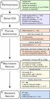
Figure 1
Figure 1
Schematic of the analysis pipeline. Boxes on the left indicate general steps potentially applicable to a variety of data and analysis types; boxes on the right indicate particular choices made for the data and analysis presented here. See Section 2 for details and abbreviations.
Figure 2
Figure 2
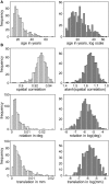
Distributions of continuous covariates of interest (A) and nuisance predictors (B). Distributions of covariates are skewed (light gray, left panels) so are transformed to have more symmetric distributions (dark gray, right panels). This reduces disproportionate influence of more extreme observations on the MANCOVA and univariate model fits.
Figure 3
Figure 3
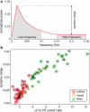
Spectral characteristics of component TCs. (A) Average power spectrum of independent component (IC) 52 illustrating the features used to compute dynamic range and low frequency (LF) to high frequency (HF) power ratio. (B) Scatter plot of LF to HF power ratio versus dynamic range for all components. Along with spectral characteristics, SMs were used to categorize components as RSNs (green), artifacts (red) or mixture of the two (yellow).
Figure 4
Figure 4
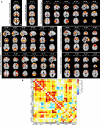
Functional connectivity within and between RSNs. (A) SMs of the 28 components identified as RSNs. SMs are plotted as t-statistics, thresholded at tc > μc + 4σc (see Appendix B), and are displayed at the three most informative slices. RSNs are divided into groups based on their anatomical and functional properties and include basal ganglia (BG), auditory (AUD), sensorimotor (MOT), visual (VIS), default-mode (DMN), attentional (ATTN), and frontal (FRONT) networks. (B) Functional network connectivity matrix. Pairwise correlations between RSN TCs were Fisher z-transformed and averaged across subjects, then inverse z-transformed for display.
Figure 5
Figure 5
Results from the reduced MANCOVA models, depicting the significance of covariates of interest (top) and nuisance predictors (bottom) for power spectra (left), SMs (middle), and the FNC matrix (right) in log10(p) units. White cells indicate terms that were removed from the full model during backward selection process. Note that the term labels refer to continuous covariates following normalizing transformations (e.g., log(age); see Figure 2). Also note that the range of log10(p) is limited by computational precision. In our analysis, epsilon is 2−52, which corresponds to a maximal −log10(p) value of 15.65.
Figure 6
Figure 6
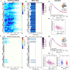
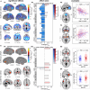
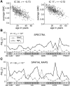
Univariate test results showing the effects of age (A) and gender (B) on power spectra. Univariate tests were performed only on covariates of interest retained in the reduced MANCOVA model (Figure 5). Left panels (A1,B1) depict the significance and direction of age (A) and gender (B) terms as a function of frequency for each component, displayed as the −sign(t)log10(p). Dashed horizontal lines on the colorbar designate the FDR-corrected threshold (α = 0.01). Middle panels (A2,B2) show bar plots of the average β-values for age (A) and gender (B) terms. β-Values were averaged over frequency bands with effects of the same directionality where test statistics exceeded the FDR threshold. The color of the bar is proportional to the fraction of contributing frequency bins; the absence of a bar indicates that univariate tests were not performed or test statistics were not significant. Right panels show examples of components with a sole age effect (A, IC 53, posterior DMN) and both age and gender effects (B, IC 72, precuneus). Line plots of the power spectra (A3,B3) show the mean log(power) ± 1 SE for males (blue) and females (red). Horizontal bars on the frequency axis denote bands with significant effects for age (white bar, solid line) and gender (gray bar, dotted line), and correspond to the range over which log(power) was averaged in the scatter plots. Scatter plots (A4, B4) show the covariate of interest versus log(power) after adjusting for nuisance regressors and age (for gender effects). The model fit is shown by colored lines and squares for age and gender, respectively. We indicate the number of frequency bins contributing to the data displayed (b) and the partial correlation coefficient (rp) between the covariate of interest and log(power).
Figure 7
Figure 7
Univariate test results showing the effects age (A) and gender (B) on SMs, in a similar format to Figure 6. Left panels (A1,B1) show surface and volumetric maps depicting composite renderings of significant effects over all RSNs, displayed as the −sign(t)log10(p). Effects are considered significant if test statistics exceeded the FDR threshold (α = 0.01) with a cluster extent of at least 27 contiguous voxels. Middle panels (A2,B2) show bar plots of the average β-values for the age (A2) and gender (B2) terms. β-Values were averaged over significant clusters with effects of the same directionality and the color of the bar is proportional to the fraction of component voxels contributing to each effect. Right panels show examples of components with age effects (A3: IC 25, anterior DMN, and A4: IC 21, basal ganglia,) and gender effects (B3: IC 21, basal ganglia, and B4: IC 20, left IFG). Scatter plots show the effects for a single significant cluster (indicated by asterisks in the −sign(t) log10(p) maps), with the number of contributing voxels indicated on each plot (V).
Figure 8
Figure 8
Univariate test results showing the effects age (A) and gender (B) on FNC, in a similar format to Figure 6. Top panels depict the significance and direction of age (A1) and gender (B1) terms for each pairwise correlation, displayed as the −sign(t)log10(p). Dashed horizontal lines on the colorbar designate the FDR-corrected threshold (α = 0.01). Bottom panels show examples of age effects (A2, temporal correlation (k) between motor RSNs IC 38 and IC 56) and both age and gender effects (B2, between motor RSN IC 24 and precuneus RSN IC 72). FNC examples are highlighted in panels (A1,B1) by asterisks.
Figure A1
Figure A1
A typical example of the normal-gamma-gamma (NGGs) model, fit to the distribution of t-statistics for IC 38. The distribution (gray) is relatively well described by a mixture of a normal (green), positive gamma (red), and negative gamma (blue). The full model fit is shown in black, and cutoffs (μ ± 4σ) are determined from the estimated mean (μ) and SD (σ) of the normal. Thresholded SMs include only voxels with positive t-statistics: t > μ + 4σ.
Figure A2
Figure A2
Evaluation of age and gray matter concentration as predictors. (A) Typical examples of the relationship between log(age) and GMC (averaged over voxels in the thresholded SM). (B,C) Significance of the residualized GMC (GMCr, gray) and residualized log(age; ager, black) terms in models predicting spectral power (B) and SM intensity (C) for each RSN. Wilcoxon signed-rank statistics (W), based on the difference between −log10(p) values, are displayed on each plot.
Figure A3
Figure A3
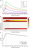
Simulations showing benefits of dimension reduction using the MDL estimate. (A) Average p-values from the MANCOVA F-test for each model term over different number of components used, ranging from 1 to 100. Dashed black line shows the true number of dimensions estimated correctly as 13 by MDL for all 100 simulations. (B) Hit rate (fraction of times each model term appeared in the reduced model, following backward selection) as a function of components used. (C) True positives (average hit rate for true effects) and false positives (average hit rate for false effects) as a function of components used. Though difficult to see given the scale, the false positive rate was lowest at 11 and 13 components (0.0067 and 0.0078, respectively), and never rose above 0.024 (21 components).
Figure A4
Figure A4
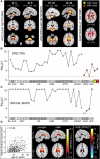
Comparison of age effects in RSN and non-RSN components. (A) SMs of components representing vascular (VASC, left panel) and ventricular (VENT, middle panel) networks. SMs are plotted as t-statistics following the format of Figure 4. Right panel shows the CSF (green) and WM (red) masks used to determine the ROI time series; see text for details. (B,C) F-test results of log(age) from the reduced MANCOVA models. −log10(p) values indicate the significance of age in predicting power spectra (B) and SMs (C) of RSNs (gray circles) and non-RSNs (orange squares). Note that for power spectra, non-RSNs comprise manually identified components (ICs 3, 6, 16, 44) as well as anatomically defined CSF (green) and WM (red) regions. When the log(age) was removed from the model during backward selection, the symbol is displayed at the significance threshold (α = 0.01, dashed line; IC 16 spectra; IC 3 SM). Note that the saturation of −log10(p) values is due to limited computational precision; for our analysis, epsilon is 2−52 thus −log10(p) is maximally 15.65. (D) Origin of significant age effect for the SM of IC 44 (lateral ventricles). Left panel: scatter plot of age versus lateral ventricular volume, as determined from the CSF segmented images with a probability threshold of 0.95. Middle panel: SMs of IC 44, averaged over the youngest quartile (<17 years, n = 134) and oldest quartile (>28 years, n = 137) of subjects. Right panel: statistical map of univariate results for IC 44 following the format of Figure 7. With age, the component distribution expands more posteriorly, increasing SM intensity in the trigone of the lateral ventricles and decreasing intensity in the frontal horns.

Similar articles

Cited by

References

    1. Abbott C., Kim D., Sponheim S. R., Bustillo J., Calhoun V. D. (2010). Decreased default mode neural modulation with age in schizophrenia. Am. J. Geriatr. Psychiatry 18, 897–907 - PMC - PubMed
    1. Abou-Elseoud A., Starck T., Remes J., Nikkinen J., Tervonen O., Kiviniemi V. (2010). The effect of model order selection in group PICA. Hum. Brain Mapp. 31, 1207–1216 - PMC - PubMed
    1. Albert N., Robertson E., Miall R. (2009). The resting human brain and motor learning. Curr. Biol. 19, 1023–1027 - PMC - PubMed
    1. Allen E., Erhardt E., Eichele T., Mayer A. R., Calhoun V. D. (2010). “Comparison of pre-normalization methods on the accuracy of group ICA results”, in 16th Annual Meeting of the Organization for Human Brain Mapping, 6–10 June, Barcelona, Spain
    1. Ances B., Liang C., Leontiev O., Perthen J., Fleisher A., Lansing A., Buxton R. (2009). Effects of aging on cerebral blood flow, oxygen metabolism, and blood oxygenation level dependent responses to visual stimulation. Hum. Brain Mapp. 30, 1120–113210.1002/hbm.20574 - DOI - PMC - PubMed