iBet uBet web content aggregator. Adding the entire web to your favor.


Link to original content: http://pubmed.ncbi.nlm.nih.gov/23675360/
Prediction, postdiction, and perceptual length contraction: a bayesian low-speed prior captures the cutaneous rabbit and related illusions - PubMed Skip to main page content
U.S. flag

An official website of the United States government

Dot gov

The .gov means it’s official.
Federal government websites often end in .gov or .mil. Before sharing sensitive information, make sure you’re on a federal government site.

Https

The site is secure.
The https:// ensures that you are connecting to the official website and that any information you provide is encrypted and transmitted securely.

Access keys NCBI Homepage MyNCBI Homepage Main Content Main Navigation
. 2013 May 10:4:221.
doi: 10.3389/fpsyg.2013.00221. eCollection 2013.

Prediction, postdiction, and perceptual length contraction: a bayesian low-speed prior captures the cutaneous rabbit and related illusions

Affiliations

Prediction, postdiction, and perceptual length contraction: a bayesian low-speed prior captures the cutaneous rabbit and related illusions

Daniel Goldreich et al. Front Psychol. .

Abstract

Illusions provide a window into the brain's perceptual strategies. In certain illusions, an ostensibly task-irrelevant variable influences perception. For example, in touch as in audition and vision, the perceived distance between successive punctate stimuli reflects not only the actual distance but curiously the inter-stimulus time. Stimuli presented at different positions in rapid succession are drawn perceptually toward one another. This effect manifests in several illusions, among them the startling cutaneous rabbit, in which taps delivered to as few as two skin positions appear to hop progressively from one position to the next, landing in the process on intervening areas that were never stimulated. Here we provide an accessible step-by-step exposition of a Bayesian perceptual model that replicates the rabbit and related illusions. The Bayesian observer optimally joins uncertain estimates of spatial location with the expectation that stimuli tend to move slowly. We speculate that this expectation - a Bayesian prior - represents the statistics of naturally occurring stimuli, learned by humans through sensory experience. In its simplest form, the model contains a single free parameter, tau: a time constant for space perception. We show that the Bayesian observer incorporates both pre- and post-dictive inference. Directed spatial attention affects the prediction-postdiction balance, shifting the model's percept toward the attended location, as observed experimentally in humans. Applying the model to the perception of multi-tap sequences, we show that the low-speed prior fits perception better than an alternative, low-acceleration prior. We discuss the applicability of our model to related tactile, visual, and auditory illusions. To facilitate future model-driven experimental studies, we present a convenient freeware computer program that implements the Bayesian observer; we invite investigators to use this program to create their own testable predictions.

Keywords: Kalman smoothing; motion illusions; optimal percepts; probabilistic inference; sensory saltation; sensory uncertainty; somatosensory spatiotemporal perception; tactile spatial attention.


Figures

Figure 1
Figure 1
Perceptual length contraction. Perception underestimates the distance between successive taps to the skin. Stimuli on the forearm are illustrated in the upper panels, along with their perception (forearm sketches). Corresponding human data and Bayesian model fits are plotted in the lower panels. In this and subsequent figures, we illustrate stimulus sequences that progress distally on the arm; the illusions occur also for stimuli in the opposite direction. (A) Top: at short ISI (t), the perceived length (l*) between two taps to the forearm is less than the actual length (l). Bottom: perceived length grows linearly with actual length, but with a slope less than 1. Filled circles: human perceptual data from Marks et al. (1982) for electrocutaneous stimuli delivered at t = 0.24 s. Solid line: fit of the Bayesian model. Dashed line: l = l*. (B) Top: a pair of taps delivered to the right forearm at short ISI (t2) is perceived to have the same spacing as a more closely spaced pair of taps (l1 < l2) delivered to the left forearm at longer ISI (t1 > t2). Bottom: the spacing ratio, l2-to-l1, resulting in perceived equality of spacing on the two arms, as a function of the ISI ratio, t1-to-t2. Filled circles: human perceptual data from Lechelt and Borchert (1977). Curve: fit of the Bayesian model. Data points from left to right had t1 = 0.2, 0.35, 0.5, 0.65, and 0.8 s, with t2 = 1.0 s − t1, and l1 = 10 cm. (C) Top: 4 taps delivered to two skin sites are perceived as hopping sequentially along the arm, because the short ISI (t) between taps 2 and 3 results in contraction of the perceived distance between them (l* < l). Bottom: the perceived length from taps 2–3 asymptotically approaches the actual length (l = 10 cm, dashed line) as ISI is increased. Filled circles: human perceptual data from Kilgard and Merzenich (1995). Curve: fit of the Bayesian model.
Figure 2
Figure 2
Bayesian model. (A) The observer’s likelihood function, prior probability density, and posterior probability density in response to taps sensed (i.e., measured by the observer) at positions (x1m, x2m) = (3, 7 cm) (open red circles in all plots). Each pixel in the intensity plots represents a candidate trajectory: a possible tap 1 position and tap 2 position pair (x1, x2). Lighter color indicates higher probability (each plot is individually auto-scaled to take advantage of the full brightness range). The measured trajectory length is lm = x2m − x1m = 4 cm. Top: the observer’s likelihood function plots the probability of the measured trajectory given each candidate trajectory. The observer understands that a single tap at any location produces a measurement drawn from a Gaussian distribution centered at that location, with standard deviation σs; thus, the likelihood function is a two-dimensional Gaussian density centered on the measured trajectory. Middle: the observer expects slow movement to occur more commonly; we model this expectation as a Gaussian distribution over trajectory speed, with mean zero and standard deviation, σv. Consequently, the observer expects closely spaced taps, and its prior is maximal along the x1 = x2 diagonal. Bottom: the posterior probability of each trajectory is proportional to the product of its likelihood and prior. The mode of the posterior (filled red circle) is the percept. (B) Space-time plots equivalently illustrate the inference process. Top: open red circles show measured tap positions (vertical-axis) and times of occurrence (horizontal-axis). Error bars (±1σs) represent the spatial imprecision of the measurements. The slope of the line connecting the taps is the measured trajectory speed: lm /t = 4 cm/0.15 s = 27 cm/s. Middle: the observer’s low-speed expectation is represented by the line of slope zero and diagonal lines of slopes ±1σv = ±10 cm/s. The distance traversed at speed σv in time t is tσv = 1.5 cm. The ascending diagonal line is shallower than the measured velocity: 10 cm/s < 27 cm/s. Equivalently, tσv = 1.5 cm < lm = 4 cm. Thus, the measured trajectory violates the observer’s low-speed expectation. Bottom: the perceived trajectory (filled red circles and red line) is a compromise between the measured trajectory (open circles, reproduced from top panel) and expectation (middle panel). Each tap has migrated perceptually by 1 cm toward the other, resulting in perceptual length contraction: l* = 2cm < lm = 4 cm. The perceived trajectory speed is l*/t = 2 cm/0.15 s = 13 cm/s. In both panels, σs = 1 cm, σv = 10 cm/s, t = 0.15 s, x1m = 3 cm, x2m = 7 cm.
Figure 3
Figure 3
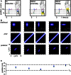
Time affects space perception. (A) The columns display the observer’s likelihood function, prior probability density, and posterior probability density on four trials in which the measured trajectory (open red circle in all plots) was x1m = 3 cm, x2m = 7 cm, and the time, t, between taps was (left to right) 0.05, 0.15, 0.25, and 0.35 s. Because the observer has a low-speed expectation, it most strongly expects the taps to fall close together when the time between them is short; thus, the narrowest prior distribution is found in the left column, and the prior distribution widens as t increases. The perceived trajectory (mode of the posterior, filled red circle) is pulled closer to the x1 = x2 diagonal when the prior is sharper. Therefore, the observer experiences more pronounced length contraction as t decreases. Conversely, as t increases, length contraction diminishes, and the perceived trajectory asymptotically approaches the measured trajectory (note diminishing distance between filled and open circles in the posterior plots as t increases). For all columns, σs = 1 cm, σv = 10 cm/s. (B) The perceived first and second tap positions (filled red circles), corresponding to the mode of each of the posterior plots above, are graphed along with the measured tap positions (dashed lines). The perceived distance between taps asymptotically approaches the measured distance as t increases (compare to Figure 1C, lower). (C) The amount of perceptual length contraction depends not only on t and σv but also on σs. Here we simulate a trial at t = 0.1 s for an observer whose spatial acuity is worse (σs = 2 cm) than the observer in (A). Although its posterior density is broader, this observer has the same percept (mode of the posterior) as the observer in (A) with t = 0.05 s (leftmost column in A). Note that the ratio of σs to σvt is identical (=2) in the two cases. It is this ratio that determines the amount of perceptual length contraction.
Figure 4
Figure 4
Perceived distance grows linearly with measured distance. (A) The columns display the observer’s likelihood function, prior probability density, and posterior probability density on five trials, in which the measured distance was progressively increased from 2 to 6 cm while t was held constant at 0.1 s. The mode of the posterior (filled red circle) tracks but lags the measured trajectory (open red circle). To facilitate comparison, yellow crosshairs in all posterior plots mark the posterior mode in the leftmost column. (B) The measurements, x1m and x2m, are plotted as open circles; the observer’s percept (mode of the posterior), as filled circles. l* grows linearly with, but consistently underestimates, lm (compare to Figure 1A, lower). The measurements (x1m, x2m) were, from left to right: (4, 6 cm), (3.5, 6.5 cm), (3, 7 cm), (2.5, 7.5 cm), and (2, 8 cm). In all panels, σs = 1 cm, σv = 10 cm/s.
Figure 5
Figure 5
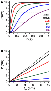
Exploring the perceptual length contraction formula. (A) Perceived length, l*, plotted against ISI (t), for a trajectory of measured length lm = 10 cm, at five values of the parameter τ (Eq. 2). Perceived length asymptotically approaches measured length as t increases. Each curve reaches l* = (1/3) lm (lower dashed line) when t = τ, and l* = (2/3) lm (upper dashed line) when t = 2τ. (B) Perceived length, l*, plotted against measured length, lm, for a trajectory of t = 0.1 s, at five values of τ [color code as in (A)]. Perceived length grows linearly with, but underestimates, measured length. Observers with larger τ experience more pronounced length contraction. Dashed diagonal line: l* = lm.
Figure 6
Figure 6
Measurement noise causes stochastic perception. (A) The columns display the observer’s likelihood function, prior probability distribution, and posterior probability distribution on five trials with the identical stimulus trajectory: x1 = 3 cm, x2 = 7 cm, t = 0.15 s. Each measured stimulus position was randomly sampled from the true location; thus, the measured trajectory (x1m, x2m; open red circle) bounces randomly from trial to trial around the fixed true value (3, 7 cm; red cross). Because the likelihood function is centered on the measurement, it too bounces. Consequently, the observer’s percept (mode of the posterior, filled red circle) varies stochastically from trial to trial. (B) The measured tap positions (open circles) and perceived tap positions (mode of posterior, filled red circles) on each trial, compared to the actual tap positions (dashed lines). On every trial, the perceived trajectory length (l*, distance between filled circles) underestimates the measured length (lm, distance between open circles); the perceived trajectory length therefore on average underestimates the actual trajectory length (l).
Figure 7
Figure 7
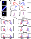
Bayesian perception is optimal because it is biased. On each of 1 million trials, a first tap position (x1) was drawn from a uniform distribution, and a second tap position (x2) was drawn from a Gaussian distribution centered on the first tap position, with standard deviation tσv = 1.5 cm (i.e., σv = 10 cm/s, t = 0.15 s; see Eq. A8 in Appendix). Measured positions, x1m and x2m, were then drawn independently from Gaussian distributions of standard deviation σs = 1 cm, centered on the corresponding tap positions (x1 and x2). (A) Left: scatterplot of measured trajectory length (lm = x2m −  x1m) against actual trajectory length (l = x2 − x1) for each of the trials (dots); negative lengths indicate trajectories in which x2 < x1. Dashed vertical and horizontal lines: l = 0 and lm = 0. Diagonal dashed line: lm = l. Vertical blue line: l = 3 cm. Horizontal red line: lm = 3 cm. Center: histogram (h) of lm values that occurred when l was between 2.95 and 3.05 cm (i.e., lm samples that fell along the blue vertical line in the scatterplot). The histogram is a Gaussian distribution centered at lm = 3 cm (asterisk). Right: histogram of l values of trajectories that gave rise to lm between 2.95 and 3.05 cm (i.e., l samples that fell along the red horizontal line in the scatterplot). The histogram represents the observer’s posterior density over l. It is a Gaussian distribution centered at l = 1.6 cm, not 3 cm (asterisk). (B) Left, center, and right panels as in (A), but for l* rather than lm. Center: l* is a biased estimator. Right: on trials in which the observer perceived l* = 3 cm, the true trajectory length averaged 3 cm. Because the perceived length is a deterministic function of the measurement, this histogram has the same variance as the posterior density over l. Inset formulas in (A) center and (B) right show the variances of these histograms (See “One-dimensional reductions” in Appendix). These are equal to the mean-squared error between each estimator and the true length.
Figure 8
Figure 8
Modeling the effects of spatial attention. (A) Depiction of a cutaneous rabbit illusion experiment reported by Kilgard and Merzenich (1995). Participants either received no specific instruction or were instructed to direct their attention (yellow highlight) toward the proximal or distal forearm. The investigators found that in the directed attention conditions, the perceived positions of tap 2 (green) and tap 3 (blue) were shifted toward the attended location (forearm sketches). (B) In the Bayesian observer, a reduction in σs at the attended relative to the unattended location reproduces the perceptual shift reported by Kilgard and Merzenich (1995). Left panel: the Bayesian observer’s likelihood function, prior and posterior density when σs does not vary with location, simulating the no-instruction condition in (A). In this case, the perceived and measured trajectory midpoints coincide. Center two panels: effect of σsp < σsd, where the subscripts p and d refer to the proximal and distal arm areas. The greater the reduction of σsp relative to σsd, the more the perceived trajectory migrates proximally toward the tap 2 measurement. Right two panels: effect of σsd < σsp. The greater the reduction of σsd relative to σsp, the more the perceived trajectory migrates distally toward the tap 3 measurement. For all plots in (B), the measurements (x2m, x3m) were (3, 7 cm), the time between taps 2 and 3 was 0.06 s, and σv was 10 cm/s. (C) The perceived (mode of posterior) tap 2 and 3 positions (green and blue circles) for each of the five conditions in (B) directly above, compared to the measured tap positions (dashed lines).
Figure 9
Figure 9
Prediction-postdiction formulation. (A) The observer’s two-dimensional joint (x1, x2) likelihood function, prior and posterior densities. The measured trajectory was x1m = 3 cm, x2m = 7 cm, with t = 0.15 s. The observer settings were σs = 1 cm, σv = 10 cm/s. (B) The inference process in (A) reformulated as a series of one-dimensional inferences regarding x1 and x2 individually. Top left: the tap 1 likelihood function (red), p(x1m | x1), is centered on x1m. Because of its low-speed expectation, the observer predicts (red arrow) that the most probable position for a future tap 2 will also be 3 cm. Middle right: the observer’s predicted prior over tap 2 (light red) represents its belief concerning the position of tap 2, projected 150 ms forward in time from the occurrence of tap 1. Top right: the observer’s tap 2 likelihood function (blue), p(x2m | x2), is centered on x2m. Because of its low-speed expectation, the observer postdicts (blue arrow) that the most probable position for the preceding tap 1 was also 7 cm. Middle left: the observer’s postdicted prior over tap 1 (light blue) represents its belief concerning the position of tap 1, projected 150 ms backward in time from the occurrence of tap 2. Left column: using Bayes’ theorem, the observer multiplies the tap 1 likelihood function (red) by the tap 1 postdicted prior (light blue) to obtain the tap 1 posterior (purple). Right column: similarly, the observer multiplies the tap 2 likelihood function (blue) by the tap 2 predicted prior (light red) to obtain the tap 2 posterior (purple). (C) Individual tap likelihoods, priors, and posteriors graphed with the same color scheme as in (B), for three trajectories of progressively increasing ISI. At t = 0.05 s, pre- and postdiction both result in relatively sharp priors that exert a strong influence over the percept (mode of the posterior). As t is increased, the pre- and postdicted priors become lower and broader: pre- and postdiction become increasingly uncertain with the passage of time. The priors thus exert diminishing influence, and the percept approaches the measurement (compare to Figure 3A). For all panels in (C), σs = 1 cm, σv = 10 cm/s. (D) Effect of directed spatial attention, as in Figure 8. Top: a reduction in σs1 sharpens the tap 1 likelihood function, increasing the strength of prediction (note sharp predicted prior over tap 2), while an increase in σs2 broadens the tap 2 likelihood function, decreasing the strength of postdiction (note broad postdicted prior over tap 1). Middle: when σs1 = σs2, pre- and postdiction have equal strength. Bottom: reduction in σs2 relative to σs1 results in effects opposite those seen in the top panel. For all panels in (D), t = 0.06 s, σv = 10 cm/s.
Figure 10
Figure 10
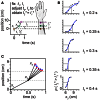
The tau effect. (A) Three taps to the arm, at positions x1 = 0 cm, x2 = 3 cm, and x3 (variable), define two spatial intervals, l1 = 3 cm and l2 (variable), and two temporal intervals, t1 = 0.5 s and t2 (variable). Because t2 < t1, at some l2 > l1 the two intervals will be perceived to be of equal length (l2* = l1*). (B) At each of five t2 settings (identified at right of plots), Helson and King (1931) progressively increased l2 by shifting x3 along the arm in 0.5-cm increments. On each trial, the participant reported whether the second spatial interval was perceived to be shorter than, equal to, or longer than the first interval. To accurately estimate each participant’s point of subjective equality (PSE), we transformed these data into a two-alternative forced-choice format by distributing the participant’s “equal” responses evenly to the “shorter” and “longer” response categories. We then fit each participant’s transformed data (proportion “l2 is longer” responses) at each t2 setting with a Weibull psychometric function (blue curves). Each psychometric function provides a PSE (vertical line): the x3 at which the psychometric function intersected 0.5 (horizontal line), indicating that l2* = l1*. The PSE shifted progressively to the left as t2 was increased (note: when x3 = 6 cm, l2 actually does equal l1). The transformed data shown are from one participant (“Observer C”) in Helson and King (1931). (C) Trajectories for which l2* = l1*. Blue points: mean x3 that resulted in l2* = l1* among the six participants tested by Helson and King (1931), at each of the five t2 settings. Blue lines: ±1 SD. Red points: best-fit performance of the Bayesian low-speed observer (τ = 0.10 s).
Figure 11
Figure 11
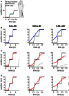
The 15-tap rabbit illusion. (A) Geldard (1982) delivered five taps at each of three locations along the arm. When ISI between successive taps was 0.05 s, participants reported perceiving a linear spatial progression of taps 1 through 10 (forearm sketch). (B) The same spatial sequence shown in (A), at three different ISIs, resulted in distinct percepts (Geldard, 1982). Left: at 0.3 s ISI, perception was veridical. Center: at 0.05 s ISI, perception was as shown in (A). Right: at 0.02 s ISI, the taps were perceived to begin at a position between 2 and 3 cm along the arm, and to advance in a non-linear spatial progression. Open circles: true tap positions; blue points: human perceptual report. (C) The Bayesian low-speed observer’s perception with a standard setting of τ = 0.10 s (e.g., σs = 1 cm, σv = 10 cm/s) shows much similarity to participants’ subjective reports. Open circles: true tap positions; red points: Bayesian observer’s perception (mode of the posterior). Dashed slanted lines have slope 10 cm/s (i.e., 1σv). Note that the two rapid jumps in the true trajectory (from tap 5 to tap 6, and from tap 10 to tap 11) occur at a speed much greater than σv when the ISI is 0.05 s (center) or 0.02 s (right); thus, perceptual length contraction occurs in these cases. In contrast, at an ISI of 0.3 s (left), the trajectory does not strongly violate the observer’s low-speed expectation; thus, perception is nearly veridical. (D) The Bayesian low-speed observer’s perception can be made even closer to human reports if the value of σs varies along the arm. The observer’s percept at each ISI is shown for σs = 1, 2, and 0.5 cm around the proximal, middle, and distal arm regions, respectively. Line segments at right have length equal to 1σs at each location. The value of σv was fixed at 10 cm/s.
Figure 12
Figure 12
Comparison between the low-speed-prior and low-acceleration-prior observers. (A) The tau effect. Red points: low-speed-prior observer’s performance, reproduced from Figure 10C, and extended to 1 s on the x-axis. Purple points: low-acceleration-prior observer’s performance. (B) The 15-tap rabbit. Red points: low-speed-prior observer’s performance, reproduced from Figure 11B. Purple points: low-acceleration-prior observer’s performance. For both observers in (A) and (B), τ was set to 0.10 s (i.e., σs = 1 cm, σv = 10 cm/s).

Similar articles

Cited by

References

    1. Anton-Erxleben K., Carrasco M. (2013). Attentional enhancement of spatial resolution: linking behavioural and neurophysiological evidence. Nat. Rev. Neurosci. 14, 188–20010.1038/nrn3443 - DOI - PMC - PubMed
    1. Asai T., Kanayama N. (2012). “Cutaneous rabbit” hops toward a light: unimodal and cross-modal causality on the skin. Front. Psychol. 3:427.10.3389/fpsyg.2012.00427 - DOI - PMC - PubMed
    1. Bays P. M., Flanagan J. R., Wolpert D. M. (2006). Attenuation of self-generated tactile sensations is predictive, not postdictive. PLoS Biol. 4:e28.10.1371/journal.pbio.0040028 - DOI - PMC - PubMed
    1. Beck J. M., Latham P. E., Pouget A. (2011). Marginalization in neural circuits with divisive normalization. J. Neurosci. 31, 15310–1531910.1523/JNEUROSCI.1706-11.2011 - DOI - PMC - PubMed
    1. Blankenburg F., Ruff C. C., Deichmann R., Rees G., Driver J. (2006). The cutaneous rabbit illusion affects human primary sensory cortex somatotopically. PLoS Biol. 4:e69.10.1371/journal.pbio.0040069 - DOI - PMC - PubMed

LinkOut - more resources